������2���������������WeChat���aptao168���Vk8YcIz

SearchAdvancedHelp

(0.002 seconds)

11—20 of 802 matching pages

11: 28.14 Fourier Series

… ►The coefficients satisfy ►

28.14.4 $$q{c}_{2m+2}-\left(a-{(\nu +2m)}^2\right)c_{2m}+q{c}_{2m-2}=0,$$ $a={\lambda }_{\nu }\left(q\right),c_{2m}=c_{2m}^{\nu }(q)$,

ⓘ

Symbols:

${\lambda }_{\nu +2n}\left(q\right)$: eigenvalues of Mathieu equation, $m$: integer, $q=h^2$: parameter, $\nu$: complex parameter, $a$: parameter and $c_{2m}(q)$: coefficients

Referenced by:

item (d), item (d)

Permalink:

http://dlmf.nist.gov/28.14.E4

Encodings:

pMML, png, TeX

See also:

Annotations for §28.14 and Ch.28

… ►

28.14.5 $$\sum _{m=-\mathrm{\infty }}^{\mathrm{\infty }}{\left(c_{2m}^{\nu }(q)\right)}^2=1;$$

ⓘ

Symbols:

$m$: integer, $q=h^2$: parameter, $\nu$: complex parameter and $c_{2m}(q)$: coefficients

Referenced by:

item (d)

Permalink:

http://dlmf.nist.gov/28.14.E5

Encodings:

pMML, png, TeX

See also:

Annotations for §28.14 and Ch.28

… ►

28.14.7 $$c_{-2m}^{-\nu }(q)=c_{2m}^{\nu }(q),$$

ⓘ

Symbols:

$m$: integer, $q=h^2$: parameter, $\nu$: complex parameter and $c_{2m}(q)$: coefficients

Permalink:

http://dlmf.nist.gov/28.14.E7

Encodings:

pMML, png, TeX

See also:

Annotations for §28.14 and Ch.28

►

28.14.8 $$c_{2m}^{\nu }(-q)={(-1)}^m{c}_{2m}^{\nu }(q).$$

ⓘ

Symbols:

$m$: integer, $q=h^2$: parameter, $\nu$: complex parameter and $c_{2m}(q)$: coefficients

Permalink:

http://dlmf.nist.gov/28.14.E8

Encodings:

pMML, png, TeX

See also:

Annotations for §28.14 and Ch.28

…

12: 30.16 Methods of Computation

… ►and real eigenvalues ${\alpha }_{1,d}$, ${\alpha }_{2,d}$, $\mathrm{\dots }$, ${\alpha }_{d,d}$, arranged in ascending order of magnitude. … ►For $m=2$, $n=4$, ${\gamma }^2=10$, …which yields ${\lambda }_4^2\left(10\right)=\mathrm{13.97907\hspace{0.33em}345}$. … ►If ${\lambda }_n^m\left({\gamma }^2\right)$ is known, then ${\mathrm{𝖯𝗌}}_n^m(x,{\gamma }^2)$ can be found by summing (30.8.1). The coefficients $a_{n,r}^m({\gamma }^2)$ are computed as the recessive solution of (30.8.4) (§3.6), and normalized via (30.8.5). …

13: 28.4 Fourier Series

… ►For $n=0,1,2,3,\mathrm{\dots }$, … ►

$(a-4m^2)B_{2m}-q(B_{2m-2}+B_{2m+2})=0$ , $m=2,3,4,\mathrm{\dots }$, $a=b_{2n+2}\left(q\right)$, $B_{2m+2}=B_{2m+2}^{2n+2}(q).$

… ►

$B_{2n+2}^{2n+2}(0)=1,$

►

$B_{2m+2}^{2n+2}(0)=0,$ $n\ne m$.

… ►For fixed $s=1,2,3,\mathrm{\dots }$ and fixed $m=1,2,3,\mathrm{\dots }$, …

14: 19.3 Graphics

… ►

►

►

Figure 19.3.5: $\mathrm{\Pi }({\alpha }^2,k)$ as a function of $k^2$ and ${\alpha }^2$ for , $-2\le {\alpha }^2\le 2$. … Magnify 3D Help

►

►

►

Figure 19.3.6: $\mathrm{\Pi }(\varphi ,2,k)$ as a function of $k^2$ and ${\sin }^2\varphi$ for $-1\le k^2\le 3$, . Cauchy principal values are shown when ${\sin }^2\varphi >\frac{1}{2}$. … Magnify 3D Help

… ►

►

►

Figure 19.3.7: $K\left(k\right)$ as a function of complex $k^2$ for $-2\le \mathrm{\Re }\left(k^2\right)\le 2$, $-2\le \mathrm{\Im }\left(k^2\right)\le 2$. … Magnify 3D Help

►

►

►

Figure 19.3.8: $E\left(k\right)$ as a function of complex $k^2$ for $-2\le \mathrm{\Re }\left(k^2\right)\le 2$, $-2\le \mathrm{\Im }\left(k^2\right)\le 2$. … Magnify 3D Help

►

►

►

Figure 19.3.9: $\mathrm{\Re }\left(K\left(k\right)\right)$ as a function of complex $k^2$ for $-2\le \mathrm{\Re }\left(k^2\right)\le 2$, $-2\le \mathrm{\Im }\left(k^2\right)\le 2$. … Magnify 3D Help

…

15: 10.53 Power Series

… ►

10.53.1 $${𝗃}_n\left(z\right)=z^n\sum _{k=0}^{\mathrm{\infty }}\frac{{(-\frac{1}{2}{z}^2)}^k}{k!(2n+2k+1)!!},$$

ⓘ

Symbols:

$!!$: double factorial, $!$: factorial (as in $n!$), ${𝗃}_n\left(z\right)$: spherical Bessel function of the first kind, $n$: integer, $k$: nonnegative integer and $z$: complex variable

A&S Ref:

10.1.2

Referenced by:

§10.53

Permalink:

http://dlmf.nist.gov/10.53.E1

Encodings:

pMML, png, TeX

See also:

Annotations for §10.53 and Ch.10

►

10.53.2 $${𝗒}_n\left(z\right)=-\frac{1}{z^{n+1}}\sum _{k=0}^n\frac{(2n-2k-1)!!{(\frac{1}{2}{z}^2)}^k}{k!}+\frac{{(-1)}^{n+1}}{z^{n+1}}\sum _{k=n+1}^{\mathrm{\infty }}\frac{{(-\frac{1}{2}{z}^2)}^k}{k!(2k-2n-1)!!}.$$

ⓘ

Symbols:

$!!$: double factorial, $!$: factorial (as in $n!$), ${𝗒}_n\left(z\right)$: spherical Bessel function of the second kind, $n$: integer, $k$: nonnegative integer and $z$: complex variable

A&S Ref:

10.1.3

Referenced by:

§10.53

Permalink:

http://dlmf.nist.gov/10.53.E2

Encodings:

pMML, png, TeX

See also:

Annotations for §10.53 and Ch.10

►

10.53.3 $${𝗂}_n^{(1)}\left(z\right)=z^n\sum _{k=0}^{\mathrm{\infty }}\frac{{(\frac{1}{2}{z}^2)}^k}{k!(2n+2k+1)!!},$$

ⓘ

Symbols:

$!!$: double factorial, $!$: factorial (as in $n!$), ${𝗂}_n^{(1)}\left(z\right)$: modified spherical Bessel function, $n$: integer, $k$: nonnegative integer and $z$: complex variable

A&S Ref:

10.2.5

Referenced by:

§10.53

Permalink:

http://dlmf.nist.gov/10.53.E3

Encodings:

pMML, png, TeX

See also:

Annotations for §10.53 and Ch.10

►

10.53.4 $${𝗂}_n^{(2)}\left(z\right)=\frac{{(-1)}^n}{z^{n+1}}\sum _{k=0}^n\frac{(2n-2k-1)!!{(-\frac{1}{2}{z}^2)}^k}{k!}+\frac{1}{z^{n+1}}\sum _{k=n+1}^{\mathrm{\infty }}\frac{{(\frac{1}{2}{z}^2)}^k}{k!(2k-2n-1)!!}.$$

ⓘ

Symbols:

$!!$: double factorial, $!$: factorial (as in $n!$), ${𝗂}_n^{(2)}\left(z\right)$: modified spherical Bessel function, $n$: integer, $k$: nonnegative integer and $z$: complex variable

A&S Ref:

10.2.6

Referenced by:

§10.53

Permalink:

http://dlmf.nist.gov/10.53.E4

Encodings:

pMML, png, TeX

See also:

Annotations for §10.53 and Ch.10

►For ${𝗁}_n^{(1)}\left(z\right)$ and ${𝗁}_n^{(2)}\left(z\right)$ combine (10.47.10), (10.53.1), and (10.53.2). …

16: 28.16 Asymptotic Expansions for Large $q$

… ►Let $s=2m+1$, $m=0,1,2,\mathrm{\dots }$, and $\nu$ be fixed with . … ►

28.16.1 $${\lambda }_{\nu }\left(h^2\right)\sim -2h^2+2sh-\frac{1}{8}(s^2+1)-\frac{1}{2^{7}h}(s^3+3s)-\frac{1}{2^{12}{h}^2}(5s^4+34s^2+9)-\frac{1}{2^{17}{h}^3}(33s^5+410s^3+405s)-\frac{1}{2^{20}{h}^4}(63s^6+1260s^4+2943s^2+486)-\frac{1}{2^{25}{h}^5}(527s^7+15617s^5+69001s^3+41607s)+\mathrm{\cdots }.$$

ⓘ

Symbols:

${\lambda }_{\nu +2n}\left(q\right)$: eigenvalues of Mathieu equation, $\sim$: Poincaré asymptotic expansion, $h$: parameter and $\nu$: complex parameter

Permalink:

http://dlmf.nist.gov/28.16.E1

Encodings:

pMML, png, TeX

See also:

Annotations for §28.16 and Ch.28

…

17: 28.6 Expansions for Small $q$

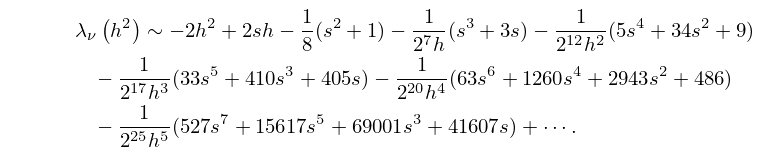
… ►For more details on these expansions and recurrence relations for the coefficients see Frenkel and Portugal (2001, §2). ►The coefficients of the power series of $a_{2n}\left(q\right)$, $b_{2n}\left(q\right)$ and also $a_{2n+1}\left(q\right)$, $b_{2n+1}\left(q\right)$ are the same until the terms in $q^{2n-2}$ and $q^{2n}$, respectively. … ►Here $j=1$ for $a_{2n}\left(q\right)$, $j=2$ for $b_{2n+2}\left(q\right)$, and $j=3$ for $a_{2n+1}\left(q\right)$ and $b_{2n+1}\left(q\right)$. … ►where $k$ is the unique root of the equation $2E\left(k\right)=K\left(k\right)$ in the interval $(0,1)$, and $k^{\prime }=\sqrt{1-k^2}$. 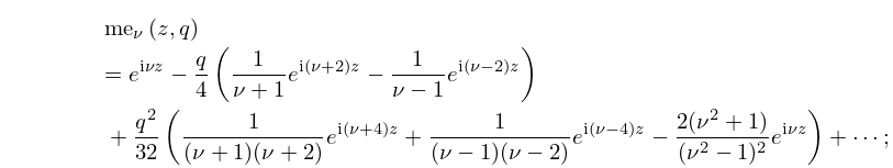… ►For more details on these expansions and recurrence relations for the coefficients see Frenkel and Portugal (2001, §2). …

18: 28.15 Expansions for Small $q$

… ►

28.15.1 $${\lambda }_{\nu }\left(q\right)={\nu }^2+\frac{1}{2({\nu }^2-1)}{q}^2+\frac{5{\nu }^2+7}{32{({\nu }^2-1)}^3({\nu }^2-4)}{q}^4+\frac{9{\nu }^4+58{\nu }^2+29}{64{({\nu }^2-1)}^5({\nu }^2-4)({\nu }^2-9)}{q}^6+\mathrm{\cdots }.$$

ⓘ

Symbols:

${\lambda }_{\nu +2n}\left(q\right)$: eigenvalues of Mathieu equation, $q=h^2$: parameter and $\nu$: complex parameter

A&S Ref:

20.3.15 (in slightly different form)

Permalink:

http://dlmf.nist.gov/28.15.E1

Encodings:

pMML, png, TeX

See also:

Annotations for §28.15(i), §28.15 and Ch.28

… ►

28.15.2 $$a-{\nu }^2-\frac{q^2}{a-{(\nu +2)}^2-}\frac{q^2}{a-{(\nu +4)}^2-}\mathrm{\cdots }=\frac{q^2}{a-{(\nu -2)}^2-}\frac{q^2}{a-{(\nu -4)}^2-}\mathrm{\cdots }.$$

ⓘ

Symbols:

$q=h^2$: parameter, $\nu$: complex parameter and $a$: parameter

Referenced by:

item (e)

Permalink:

http://dlmf.nist.gov/28.15.E2

Encodings:

pMML, png, TeX

See also:

Annotations for §28.15(i), §28.15 and Ch.28

… ►

28.15.3 $${\mathrm{me}}_{\nu }(z,q)={\mathrm{e}}^{\mathrm{i}\nu z}-\frac{q}{4}\left(\frac{1}{\nu +1}{\mathrm{e}}^{\mathrm{i}(\nu +2)z}-\frac{1}{\nu -1}{\mathrm{e}}^{\mathrm{i}(\nu -2)z}\right)+\frac{q^2}{32}\left(\frac{1}{(\nu +1)(\nu +2)}{\mathrm{e}}^{\mathrm{i}(\nu +4)z}+\frac{1}{(\nu -1)(\nu -2)}{\mathrm{e}}^{\mathrm{i}(\nu -4)z}-\frac{2({\nu }^2+1)}{{({\nu }^2-1)}^2}{\mathrm{e}}^{\mathrm{i}\nu z}\right)+\mathrm{\cdots };$$

ⓘ

Symbols:

${\mathrm{me}}_n(z,q)$: Mathieu function, $\mathrm{e}$: base of natural logarithm, $\mathrm{i}$: imaginary unit, $q=h^2$: parameter, $z$: complex variable and $\nu$: complex parameter

A&S Ref:

20.3.17 (only two terms and without normalization)

Permalink:

http://dlmf.nist.gov/28.15.E3

Encodings:

pMML, png, TeX

See also:

Annotations for §28.15(ii), §28.15 and Ch.28

…

19: 29.7 Asymptotic Expansions

… ►

$p=2m+1,$

… ►

29.7.4 $${\tau }_1=\frac{p}{2^6}({(1+k^2)}^2(p^2+3)-4k^2(p^2+5)).$$

ⓘ

Symbols:

$p$: nonnegative integer, $k$: real parameter and ${\tau }_j$: coefficients

Permalink:

http://dlmf.nist.gov/29.7.E4

Encodings:

pMML, png, TeX

See also:

Annotations for §29.7(i), §29.7 and Ch.29

►The same Poincaré expansion holds for $b_{\nu }^{m+1}\left(k^2\right)$, since … ►

29.7.6 $${\tau }_2=\frac{1}{2^{10}}(1+k^2){(1-k^2)}^2(5p^4+34p^2+9),$$

ⓘ

Symbols:

$p$: nonnegative integer, $k$: real parameter and ${\tau }_j$: coefficients

Permalink:

http://dlmf.nist.gov/29.7.E6

Encodings:

pMML, png, TeX

See also:

Annotations for §29.7(i), §29.7 and Ch.29

… ►In Müller (1966c) it is shown how these expansions lead to asymptotic expansions for the Lamé functions ${\mathrm{𝐸𝑐}}_{\nu }^m(z,k^2)$ and ${\mathrm{𝐸𝑠}}_{\nu }^m(z,k^2)$. …

20: 29.14 Orthogonality

… ►

29.14.4 $${\mathrm{𝑠𝐸}}_{2n+1}^m(s,k^2){\mathrm{𝑠𝐸}}_{2n+1}^m(K+\mathrm{i}t,k^2),$$

ⓘ

Symbols:

${\mathrm{𝑠𝐸}}_{2n+1}^m(z,k^2)$: Lamé polynomial, $K\left(k\right)$: Legendre’s complete elliptic integral of the first kind, $\mathrm{i}$: imaginary unit, $m$: nonnegative integer, $n$: nonnegative integer and $k$: real parameter

Referenced by:

§29.14

Permalink:

http://dlmf.nist.gov/29.14.E4

Encodings:

pMML, png, TeX

See also:

Annotations for §29.14 and Ch.29

►

29.14.5 $${\mathrm{𝑐𝐸}}_{2n+1}^m(s,k^2){\mathrm{𝑐𝐸}}_{2n+1}^m(K+\mathrm{i}t,k^2),$$

ⓘ

Symbols:

${\mathrm{𝑐𝐸}}_{2n+1}^m(z,k^2)$: Lamé polynomial, $K\left(k\right)$: Legendre’s complete elliptic integral of the first kind, $\mathrm{i}$: imaginary unit, $m$: nonnegative integer, $n$: nonnegative integer and $k$: real parameter

Permalink:

http://dlmf.nist.gov/29.14.E5

Encodings:

pMML, png, TeX

See also:

Annotations for §29.14 and Ch.29

… ►

29.14.7 $${\mathrm{𝑠𝑐𝐸}}_{2n+2}^m(s,k^2){\mathrm{𝑠𝑐𝐸}}_{2n+2}^m(K+\mathrm{i}t,k^2),$$

ⓘ

Symbols:

${\mathrm{𝑠𝑐𝐸}}_{2n+2}^m(z,k^2)$: Lamé polynomial, $K\left(k\right)$: Legendre’s complete elliptic integral of the first kind, $\mathrm{i}$: imaginary unit, $m$: nonnegative integer, $n$: nonnegative integer and $k$: real parameter

Permalink:

http://dlmf.nist.gov/29.14.E7

Encodings:

pMML, png, TeX

See also:

Annotations for §29.14 and Ch.29

►

29.14.8 $${\mathrm{𝑠𝑑𝐸}}_{2n+2}^m(s,k^2){\mathrm{𝑠𝑑𝐸}}_{2n+2}^m(K+\mathrm{i}t,k^2),$$

ⓘ

Symbols:

${\mathrm{𝑠𝑑𝐸}}_{2n+2}^m(z,k^2)$: Lamé polynomial, $K\left(k\right)$: Legendre’s complete elliptic integral of the first kind, $\mathrm{i}$: imaginary unit, $m$: nonnegative integer, $n$: nonnegative integer and $k$: real parameter

Permalink:

http://dlmf.nist.gov/29.14.E8

Encodings:

pMML, png, TeX

See also:

Annotations for §29.14 and Ch.29

►

29.14.9 $${\mathrm{𝑐𝑑𝐸}}_{2n+2}^m(s,k^2){\mathrm{𝑐𝑑𝐸}}_{2n+2}^m(K+\mathrm{i}t,k^2),$$

ⓘ

Symbols:

${\mathrm{𝑐𝑑𝐸}}_{2n+2}^m(z,k^2)$: Lamé polynomial, $K\left(k\right)$: Legendre’s complete elliptic integral of the first kind, $\mathrm{i}$: imaginary unit, $m$: nonnegative integer, $n$: nonnegative integer and $k$: real parameter

Permalink:

http://dlmf.nist.gov/29.14.E9

Encodings:

pMML, png, TeX

See also:

Annotations for §29.14 and Ch.29

…