也门护照样本资料【言正 微aptao168】5AYnp

SearchAdvancedHelp

(0.002 seconds)

11—20 of 286 matching pages

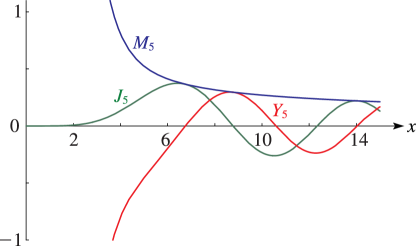
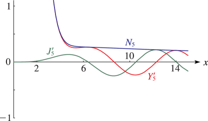
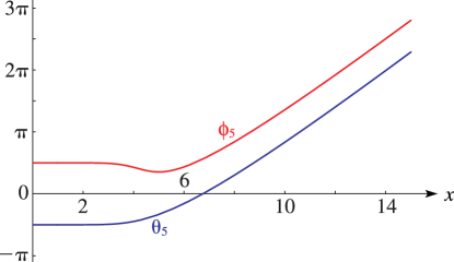
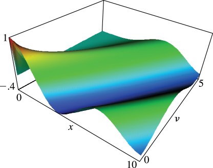
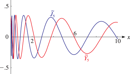
11: 10.3 Graphics

… ►

►►

Figure 10.3.2: $J_5\left(x\right)$, $Y_5\left(x\right)$, $M_5\left(x\right)$, $0\le x\le 15$. Magnify

►

►►

Figure 10.3.3: $J_5^{\prime }\left(x\right)$, $Y_5^{\prime }\left(x\right)$, $N_5\left(x\right)$, $0\le x\le 15$. Magnify

►

►►

Figure 10.3.4: ${\theta }_5\left(x\right)$, ${\varphi }_5\left(x\right)$, $0\le x\le 15$. Magnify

►

►

►

Figure 10.3.5: $J_{\nu }\left(x\right)$, $0\le x\le 10$, $0\le \nu \le 5$. Magnify 3D Help

… ►

►►

Figure 10.3.19: ${\tilde{J}}_5\left(x\right)$, ${\tilde{Y}}_5\left(x\right)$, $0.01\le x\le 10$. Magnify

12: 13.30 Tables

… ►

Zhang and Jin (1996, pp. 411–423) tabulates $M(a,b,x)$ and $U(a,b,x)$ for $a=-5(.5)5$, $b=0.5(.5)5$, and $x=0.1,1,5,10,20,30$, 8S (for $M(a,b,x)$) and 7S (for $U(a,b,x)$).

…

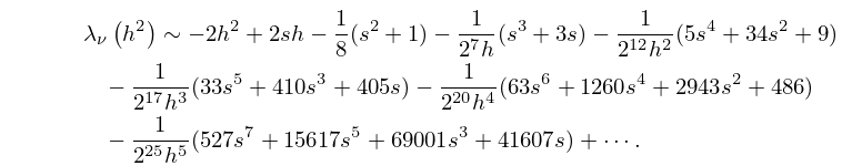
13: 28.16 Asymptotic Expansions for Large $q$

… ►

28.16.1 $${\lambda }_{\nu }\left(h^2\right)\sim -2h^2+2sh-\frac{1}{8}(s^2+1)-\frac{1}{2^{7}h}(s^3+3s)-\frac{1}{2^{12}{h}^2}(5s^4+34s^2+9)-\frac{1}{2^{17}{h}^3}(33s^5+410s^3+405s)-\frac{1}{2^{20}{h}^4}(63s^6+1260s^4+2943s^2+486)-\frac{1}{2^{25}{h}^5}(527s^7+15617s^5+69001s^3+41607s)+\mathrm{\cdots }.$$

ⓘ

Symbols:

${\lambda }_{\nu +2n}\left(q\right)$: eigenvalues of Mathieu equation, $\sim$: Poincaré asymptotic expansion, $h$: parameter and $\nu$: complex parameter

Permalink:

http://dlmf.nist.gov/28.16.E1

Encodings:

pMML, png, TeX

See also:

Annotations for §28.16 and Ch.28

…

14: Simon Ruijsenaars

… ►

5 Gamma Function

…

15: 14.33 Tables

… ►

Abramowitz and Stegun (1964, Chapter 8) tabulates ${𝖯}_n\left(x\right)$ for $n=0(1)3,9,10$, $x=0(.01)1$, 5–8D; ${𝖯}_n^{\prime }\left(x\right)$ for $n=1(1)4,9,10$, $x=0(.01)1$, 5–7D; ${𝖰}_n\left(x\right)$ and ${𝖰}_n^{\prime }\left(x\right)$ for $n=0(1)3,9,10$, $x=0(.01)1$, 6–8D; $P_n\left(x\right)$ and $P_n^{\prime }\left(x\right)$ for $n=0(1)5,9,10$, $x=1(.2)10$, 6S; $Q_n\left(x\right)$ and $Q_n^{\prime }\left(x\right)$ for $n=0(1)3,9,10$, $x=1(.2)10$, 6S. (Here primes denote derivatives with respect to $x$.)

►

Zhang and Jin (1996, Chapter 4) tabulates ${𝖯}_n\left(x\right)$ for $n=2(1)5,10$, $x=0(.1)1$, 7D; ${𝖯}_n\left(\cos \theta \right)$ for $n=1(1)4,10$, $\theta =0(5^{\circ }){90}^{\circ }$, 8D; ${𝖰}_n\left(x\right)$ for $n=0(1)2,10$, $x=0(.1)0.9$, 8S; ${𝖰}_n\left(\cos \theta \right)$ for $n=0(1)3,10$, $\theta =0(5^{\circ }){90}^{\circ }$, 8D; ${𝖯}_n^m\left(x\right)$ for $m=1(1)4$, $n-m=0(1)2$, $n=10$, $x=0,0.5$, 8S; ${𝖰}_n^m\left(x\right)$ for $m=1(1)4$, $n=0(1)2,10$, 8S; ${𝖯}_{\nu }^m\left(\cos \theta \right)$ for $m=0(1)3$, $\nu =0(.25)5$, $\theta =0({15}^{\circ }){90}^{\circ }$, 5D; $P_n\left(x\right)$ for $n=2(1)5,10$, $x=1(1)10$, 7S; $Q_n\left(x\right)$ for $n=0(1)2,10$, $x=2(1)10$, 8S. Corresponding values of the derivative of each function are also included, as are 6D values of the first 5 $\nu$-zeros of ${𝖯}_{\nu }^m\left(\cos \theta \right)$ and of its derivative for $m=0(1)4$, $\theta ={10}^{\circ },{30}^{\circ },{150}^{\circ }$.

… ►

Žurina and Karmazina (1964, 1965) tabulate the conical functions ${𝖯}_{-\frac{1}{2}+\mathrm{i}\tau }\left(x\right)$ for $\tau =0(.01)50$, $x=-0.9(.1)0.9$, 7S; $P_{-\frac{1}{2}+\mathrm{i}\tau }\left(x\right)$ for $\tau =0(.01)50$, $x=1.1(.1)2(.2)5(.5)10(10)60$, 7D. Auxiliary tables are included to facilitate computation for larger values of $\tau$ when .

►

Žurina and Karmazina (1963) tabulates the conical functions ${𝖯}_{-\frac{1}{2}+\mathrm{i}\tau }^1\left(x\right)$ for $\tau =0(.01)25$, $x=-0.9(.1)0.9$, 7S; $P_{-\frac{1}{2}+\mathrm{i}\tau }^1\left(x\right)$ for $\tau =0(.01)25$, $x=1.1(.1)2(.2)5(.5)10(10)60$, 7S. Auxiliary tables are included to assist computation for larger values of $\tau$ when .

…

16: 8.26 Tables

… ►

Pearson (1965) tabulates the function $I(u,p)$ ($=P(p+1,u)$) for $p=-1(.05)0(.1)5(.2)50$, $u=0(.1)u_p$ to 7D, where $I(u,u_p)$ rounds off to 1 to 7D; also $I(u,p)$ for $p=-0.75(.01)-1$, $u=0(.1)6$ to 5D.

►

Zhang and Jin (1996, Table 3.8) tabulates $\gamma (a,x)$ for $a=0.5,1,3,5,10,25,50,100$, $x=0(.1)1(1)3,5(5)30,50,100$ to 8D or 8S.

… ►

Zhang and Jin (1996, Table 3.9) tabulates $I_x(a,b)$ for $x=0(.05)1$, $a=0.5,1,3,5,10$, $b=1,10$ to 8D.

… ►

Stankiewicz (1968) tabulates $E_n\left(x\right)$ for $n=1(1)10$, $x=0.01(.01)5$ to 7D.

►

Zhang and Jin (1996, Table 19.1) tabulates $E_n\left(x\right)$ for $n=1,2,3,5,10,15,20$, $x=0(.1)1,1.5,2,3,5,10,20,30,50,100$ to 7D or 8S.

17: 23 Weierstrass Elliptic and Modular
Functions

…

18: 26.2 Basic Definitions

… ►If, for example, a permutation of the integers 1 through 6 is denoted by $256413$, then the cycles are $\left(1,2,5\right)$, $\left(3,6\right)$, and $\left(4\right)$. Here $\sigma (1)=2,\sigma (2)=5$, and $\sigma (5)=1$. … ►As an example, $\{1,3,4\}$, $\{2,6\}$, $\{5\}$ is a partition of $\{1,2,3,4,5,6\}$. … ►For the actual partitions ($\pi$) for $n=1(1)5$ see Table 26.4.1. … ►

Table 26.2.1: Partitions $p\left(n\right)$.

► ►►►

$n$	$p\left(n\right)$	$n$	$p\left(n\right)$	$n$	$p\left(n\right)$
…
4	5	21	792	38	26015
…

►

19: 26.9 Integer Partitions: Restricted Number and Part Size

… ►

Table 26.9.1: Partitions $p_k\left(n\right)$.

► ►►►►►

$n$	$k$
	0	1	2	3	4	5	6	7	8	9	10
…
4	0	1	3	4	5	5	5	5	5	5	5
5	0	1	3	5	6	7	7	7	7	7	7
…

►

… ►The conjugate to the example in Figure 26.9.1 is $6+5+4+2+1+1+1$. … ►

Figure 26.9.2: The partition $5+5+3+2$ represented as a lattice path.

…

20: 4.33 Maclaurin Series and Laurent Series

… ►

4.33.1 $$\sinh z=z+\frac{z^3}{3!}+\frac{z^5}{5!}+\mathrm{\cdots },$$

ⓘ

Symbols:

$!$: factorial (as in $n!$), $\sinh z$: hyperbolic sine function and $z$: complex variable

A&S Ref:

4.5.62

Permalink:

http://dlmf.nist.gov/4.33.E1

Encodings:

pMML, png, TeX

See also:

Annotations for §4.33 and Ch.4

… ►

4.33.3 $$\tanh z=z-\frac{z^3}{3}+\frac{2}{15}{z}^5-\frac{17}{315}{z}^7+\mathrm{\cdots }+\frac{2^{2n}(2^{2n}-1)B_{2n}}{(2n)!}{z}^{2n-1}+\mathrm{\cdots },$$ .

ⓘ

Symbols:

$B_n$: Bernoulli numbers, $\pi$: the ratio of the circumference of a circle to its diameter, $!$: factorial (as in $n!$), $\tanh z$: hyperbolic tangent function, $n$: integer and $z$: complex variable

A&S Ref:

4.5.64

Permalink:

http://dlmf.nist.gov/4.33.E3

Encodings:

pMML, png, TeX

See also:

Annotations for §4.33 and Ch.4

…