%E7%AB%9E%E5%BD%A9%E8%B6%B3%E7%90%83%E8%BF%87%E5%85%B3%E6%96%B9%E5%BC%8F3%C3%971%E3%80%90%E4%BA%9A%E5%8D%9A%E5%AE%98%E6%96%B9qee9.com%E3%80%91%E7%94%B5%E8%84%91%E6%AC%A2%E4%B9%90%E6%96%97%E5%9C%B0%E4%B8%BB%E5%9C%A8%E5%93%AA%E9%87%8CNuq7IN

SearchAdvancedHelp

Did you mean %E7%AB%9E%E5%BD%A9%E8%B6%B3%E7%90%83%E8%BF%87%E5%85%B3%E6%96%B9%E5%BC%8F3%C3%971%E3%80%90%E4%BA%9A%E5%8D%9A%E5%AE%98%E6%96%welcom%E3%80%91%E7%94%B5%E8%84%91%E6%AC%A2%E4%B9%90%E6%96%97%E5%9C%B0%E4%B8%BB%E5%9C%A8%E5%93%AA%E9%87%8CNuq7IN ?

(0.033 seconds)

1—10 of 552 matching pages

1: 34.6 Definition: $\mathit{9}j$ Symbol

§34.6 Definition: $\mathit{9}j$ Symbol

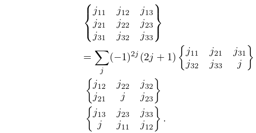
►The $\mathit{9}j$ symbol may be defined either in terms of $\mathit{3}j$ symbols or equivalently in terms of $\mathit{6}j$ symbols: ►

34.6.1

ⓘ

Defines:

: $\mathit{9}j$ symbol

Symbols:

: $\mathit{3}j$ symbol, $j,j_r$: non-negative integers or non-negative integers plus one half., $r$: nonnegative integer and $s$: integer

Permalink:

http://dlmf.nist.gov/34.6.E1

Encodings:

pMML, png, TeX

See also:

Annotations for §34.6 and Ch.34

►

34.6.2

ⓘ

Symbols:

: $\mathit{9}j$ symbol, : $\mathit{6}j$ symbol and $j,j_r$: non-negative integers or non-negative integers plus one half.

Referenced by:

§34.13

Permalink:

http://dlmf.nist.gov/34.6.E2

Encodings:

pMML, png, TeX

See also:

Annotations for §34.6 and Ch.34

►The $\mathit{9}j$ symbol may also be written as a finite triple sum equivalent to a terminating generalized hypergeometric series of three variables with unit arguments. …

2: 34.12 Physical Applications

§34.12 Physical Applications

►The angular momentum coupling coefficients ($\mathit{3}j$, $\mathit{6}j$, and $\mathit{9}j$ symbols) are essential in the fields of nuclear, atomic, and molecular physics. …$\mathit{3}j,\mathit{6}j$, and $\mathit{9}j$ symbols are also found in multipole expansions of solutions of the Laplace and Helmholtz equations; see Carlson and Rushbrooke (1950) and Judd (1976).

3: 9 Airy and Related Functions

Chapter 9 Airy and Related Functions

…

4: Bibliography C

… ►

A quadrature formula for the Hankel transform. Numer. Algorithms 9 (2), pp. 343–354.

ⓘ

External Links:

ISSN 1017-1398, Document, MathReview (V. I. Polovinkin), ZentralBlatt

Referenced by:

§10.74(vii).

Encodings:

BibTeX

… ►

Short proofs of three theorems on elliptic integrals. SIAM J. Math. Anal. 9 (3), pp. 524–528.

ⓘ

External Links:

Document, MathReview (Y. L. Luke), ZentralBlatt

Referenced by:

§19.26(i).

Encodings:

BibTeX

… ►

Extremal measures for a system of orthogonal polynomials. Constr. Approx. 9, pp. 111–119.

ⓘ

External Links:

ISSN 0176-4276, Document, MathReview (Mizan Rahman), ZentralBlatt

Referenced by:

§18.28(iv).

Encodings:

BibTeX

… ►

A moment problem and a family of integral evaluations. Trans. Amer. Math. Soc. 358 (9), pp. 4071–4097.

ⓘ

External Links:

ISSN 0002-9947, Document, MathReview (Roelof Koekoek), ZentralBlatt

Referenced by:

§18.28(iv).

Encodings:

BibTeX

… ►

Nonclassical Symmetry Reductions and Exact Solutions for Physically Significant Nonlinear Evolution Equations. In Nonlinear and Chaotic Phenomena in Plasmas, Solids and Fluids (Edmonton, AB, 1990), W. Rozmus and J. A. Tuszynski (Eds.), pp. 72–79.

ⓘ

External Links:

MathReview

Referenced by:

§29.19(ii).

Encodings:

BibTeX

…

5: 24.2 Definitions and Generating Functions

… ►

$E_{2n+1}=0$ ,

… ►

24.2.9 $$E_n=2^n{E}_n\left(\frac{1}{2}\right)=\text{integer},$$

ⓘ

Symbols:

$E_n$: Euler numbers, $E_n\left(x\right)$: Euler polynomials and $n$: integer

A&S Ref:

23.1.2

Permalink:

http://dlmf.nist.gov/24.2.E9

Encodings:

pMML, png, TeX

See also:

Annotations for §24.2(ii), §24.2 and Ch.24

… ►

${\tilde{E}}_n\left(x\right)=E_n\left(x\right)$ , ,

… ►

${\tilde{E}}_n\left(x+1\right)=-{\tilde{E}}_n\left(x\right)$ , $x\in ℝ$.

… ►

Table 24.2.4: Euler numbers $E_n$.

► ►►

$n$	$E_n$
…

►

…

6: 8.26 Tables

… ►

Abramowitz and Stegun (1964, pp. 245–248) tabulates $E_n\left(x\right)$ for $n=2,3,4,10,20$, $x=0(.01)2$ to 7D; also $(x+n){\mathrm{e}}^x{E}_n\left(x\right)$ for $n=2,3,4,10,20$, $x^{-1}=0(.01)0.1(.05)0.5$ to 6S.

►

Chiccoli et al. (1988) presents a short table of $E_p\left(x\right)$ for $p=-\frac{9}{2}(1)-\frac{1}{2}$, $0\le x\le 200$ to 14S.

►

Pagurova (1961) tabulates $E_n\left(x\right)$ for $n=0(1)20$, $x=0(.01)2(.1)10$ to 4-9S; ${\mathrm{e}}^x{E}_n\left(x\right)$ for $n=2(1)10$, $x=10(.1)20$ to 7D; ${\mathrm{e}}^x{E}_p\left(x\right)$ for $p=0(.1)1$, $x=0.01(.01)7(.05)12(.1)20$ to 7S or 7D.

►

Stankiewicz (1968) tabulates $E_n\left(x\right)$ for $n=1(1)10$, $x=0.01(.01)5$ to 7D.

►

Zhang and Jin (1996, Table 19.1) tabulates $E_n\left(x\right)$ for $n=1,2,3,5,10,15,20$, $x=0(.1)1,1.5,2,3,5,10,20,30,50,100$ to 7D or 8S.

7: 34 3j, 6j, 9j Symbols

Chapter 34 $\mathit{3}j,\mathit{6}j,\mathit{9}j$ Symbols

…

8: 34.14 Tables

§34.14 Tables

►Tables of exact values of the squares of the $\mathit{3}j$ and $\mathit{6}j$ symbols in which all parameters are $\le 8$ are given in Rotenberg et al. (1959), together with a bibliography of earlier tables of $\mathit{3}j,\mathit{6}j$, and $\mathit{9}j$ symbols on pp. … ►Some selected $\mathit{9}j$ symbols are also given. … 16-17; for $\mathit{9}j$ symbols on p. … ► 310–332, and for the $\mathit{9}j$ symbols on pp. …

9: 19.36 Methods of Computation

… ►where the elementary symmetric functions $E_s$ are defined by (19.19.4). … ►Accurate values of $F(\varphi ,k)-E(\varphi ,k)$ for $k^2$ near 0 can be obtained from $R_D$ by (19.2.6) and (19.25.13). … ► $E(\varphi ,k)$ can be evaluated by using (19.25.7), and $R_D$ by using (19.21.10), but cancellations may become significant. Thompson (1997, pp. 499, 504) uses descending Landen transformations for both $F(\varphi ,k)$ and $E(\varphi ,k)$. … ►Lee (1990) compares the use of theta functions for computation of $K\left(k\right)$, $E\left(k\right)$, and $K\left(k\right)-E\left(k\right)$, $0\le k^2\le 1$, with four other methods. …

10: 16.26 Approximations

… ►For discussions of the approximation of generalized hypergeometric functions and the Meijer $G$-function in terms of polynomials, rational functions, and Chebyshev polynomials see Luke (1975, §§5.12 - 5.13) and Luke (1977b, Chapters 1 and 9).