%E6%BE%B3%E9%97%A8%E8%B5%8C%E5%9C%BA%E5%AE%98%E7%BD%91,%E6%BE%B3%E9%97%A8%E8%B5%8C%E5%9C%BA%E6%8E%92%E5%90%8D,%E6%BE%B3%E9%97%A8%E8%B5%8C%E5%9C%BA%E6%94%BB%E7%95%A5,%E3%80%90%E6%BE%B3%E9%97%A8%E8%B5%8C%E5%9C%BA%E7%BD%91%E5%9D%80%E2%88%B6789yule.com%E3%80%91%E6%BE%B3%E9%97%A8%E7%BD%91%E4%B8%8A%E8%B5%8C%E5%9C%BA%E6%B8%B8%E6%88%8F%E7%A7%8D%E7%B1%BB,%E6%BE%B3%E9%97%A8%E8%B5%8C%E5%9C%BA%E4%BB%8B%E7%BB%8D,%E6%BE%B3%E9%97%A8%E8%B5%8C%E5%9C%BA%E7%8E%A9%E6%B3%95,%E8%B5%8C%E5%9C%BA%E6%B8%B8%E6%88%8F%E8%A7%84%E5%88%99,%E6%BE%B3%E9%97%A8%E8%B5%8C%E5%9C%BAapp,%E3%80%90%E5%8D%9A%E5%BD%A9%E7%BD%91%E5%9D%80%E2%88%B6789yule.com%E3%80%91

SearchAdvancedHelp

Did you mean %E6%BE%B3%E9%97%A8%E8%B5%8C%E5%9C%BA%E5%AE%98%E7%BD%91,%E6%BE%B3%E9%97%A8%E8%B5%8C%E5%9C%BA%E6%8E%92%E5%90%8D,%E6%BE%B3%E9%97%A8%E8%B5%8C%E5%9C%BA%E6%94%BB%E7%95%A5,%E3%80%90%E6%BE%B3%E9%97%A8%E8%B5%8C%E5%9C%BA%E7%BD%91%E5%9D%80%E2%88%caniuse.com%E3%80%91%E6%BE%B3%E9%97%A8%E7%BD%91%E4%B8%8A%E8%B5%8C%E5%9C%BA%E6%B8%B8%E6%88%8F%E7%A7%8D%E7%B1%BB,%E6%BE%B3%E9%97%A8%E8%B5%8C%E5%9C%BA%E4%BB%8B%E7%BB%8D,%E6%BE%B3%E9%97%A8%E8%B5%8C%E5%9C%BA%E7%8E%A9%E6%B3%95,%E8%B5%8C%E5%9C%BA%E6%B8%B8%E6%88%8F%E8%A7%84%E5%88%99,%E6%BE%B3%E9%97%A8%E8%B5%8C%E5%9C%papp,%E3%80%90%E5%8D%9A%E5%BD%A9%E7%BD%91%E5%9D%80%E2%88%caniuse.com%E3%80%91 ?

(0.063 seconds)

1—10 of 760 matching pages

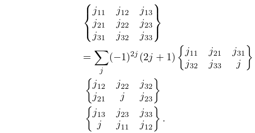
1: 34.6 Definition: $\mathit{9}j$ Symbol

§34.6 Definition: $\mathit{9}j$ Symbol

►The $\mathit{9}j$ symbol may be defined either in terms of $\mathit{3}j$ symbols or equivalently in terms of $\mathit{6}j$ symbols: ►

34.6.1

ⓘ

Defines:

: $\mathit{9}j$ symbol

Symbols:

: $\mathit{3}j$ symbol, $j,j_r$: non-negative integers or non-negative integers plus one half., $r$: nonnegative integer and $s$: integer

Permalink:

http://dlmf.nist.gov/34.6.E1

Encodings:

pMML, png, TeX

See also:

Annotations for §34.6 and Ch.34

►

34.6.2

ⓘ

Symbols:

: $\mathit{9}j$ symbol, : $\mathit{6}j$ symbol and $j,j_r$: non-negative integers or non-negative integers plus one half.

Referenced by:

§34.13

Permalink:

http://dlmf.nist.gov/34.6.E2

Encodings:

pMML, png, TeX

See also:

Annotations for §34.6 and Ch.34

►The $\mathit{9}j$ symbol may also be written as a finite triple sum equivalent to a terminating generalized hypergeometric series of three variables with unit arguments. …

2: 19.2 Definitions

… ►Let $s^2(t)$ be a cubic or quartic polynomial in $t$ with simple zeros, and let $r(s,t)$ be a rational function of $s$ and $t$ containing at least one odd power of $s$. … ►Assume $1-{\sin }^2\varphi \in ℂ\setminus (-\mathrm{\infty },0]$ and $1-k^2{\sin }^2\varphi \in ℂ\setminus (-\mathrm{\infty },0]$, except that one of them may be 0, and $1-{\alpha }^2{\sin }^2\varphi \in ℂ\setminus \{0\}$. … ►

§19.2(iv) A Related Function: $R_C(x,y)$

… ►When $x$ and $y$ are positive, $R_C(x,y)$ is an inverse circular function if and an inverse hyperbolic function (or logarithm) if $x>y$: …For the special cases of $R_C(x,x)$ and $R_C(0,y)$ see (19.6.15). …

3: 27.2 Functions

… ►Functions in this section derive their properties from the fundamental theorem of arithmetic, which states that every integer $n>1$ can be represented uniquely as a product of prime powers, …($\nu \left(1\right)$ is defined to be 0.) …It can be expressed as a sum over all primes $p\le x$: … ►is the sum of the $\alpha$th powers of the divisors of $n$, where the exponent $\alpha$ can be real or complex. Note that ${\sigma }_0\left(n\right)=d\left(n\right)$. …

4: 16.25 Methods of Computation

… ►Instead a boundary-value problem needs to be formulated and solved. See §§3.6(vii), 3.7(iii), Olde Daalhuis and Olver (1998), Lozier (1980), and Wimp (1984, Chapters 7, 8).

5: 36 Integrals with Coalescing Saddles

…

6: 10.74 Methods of Computation

… ►Furthermore, the attainable accuracy can be increased substantially by use of the exponentially-improved expansions given in §10.17(v), even more so by application of the hyperasymptotic expansions to be found in the references in that subsection. ►For large positive real values of $\nu$ the uniform asymptotic expansions of §§10.20(i) and 10.20(ii) can be used. …It should be noted, however, that there is a difficulty in evaluating the coefficients $A_k(\zeta )$, $B_k(\zeta )$, $C_k(\zeta )$, and $D_k(\zeta )$, from the explicit expressions (10.20.10)–(10.20.13) when $z$ is close to $1$ owing to severe cancellation. … ►And since there are no error terms they could, in theory, be used for all values of $z$; however, there may be severe cancellation when $|z|$ is not large compared with $n^2$. … ►Then $J_n\left(x\right)$ and $Y_n\left(x\right)$ can be generated by either forward or backward recurrence on $n$ when , but if $n>x$ then to maintain stability $J_n\left(x\right)$ has to be generated by backward recurrence on $n$, and $Y_n\left(x\right)$ has to be generated by forward recurrence on $n$. …

7: Customize DLMF

…Note: Javascript and Cookies must be enabled to support customizations.

8: 13.27 Mathematical Applications

… ►Vilenkin (1968, Chapter 8) constructs irreducible representations of this group, in which the diagonal matrices correspond to operators of multiplication by an exponential function. The other group elements correspond to integral operators whose kernels can be expressed in terms of Whittaker functions. This identification can be used to obtain various properties of the Whittaker functions, including recurrence relations and derivatives. …

9: 6.18 Methods of Computation

… ►The attainable accuracy of the asymptotic expansions can be increased considerably by exponential improvement. Also, other ranges of $\mathrm{ph}z$ can be covered by use of the continuation formulas of §6.4. … ►For example, the Gauss–Laguerre formula (§3.5(v)) can be applied to (6.2.2); see Todd (1954) and Tseng and Lee (1998). … ►Lastly, the continued fraction (6.9.1) can be used if $|z|$ is bounded away from the origin. … ► $A_0$, $B_0$, and $C_0$ can be computed by Miller’s algorithm (§3.6(iii)), starting with initial values $(A_N,B_N,C_N)=(1,0,0)$, say, where $N$ is an arbitrary large integer, and normalizing via $C_0=1/z$. …

10: 5.19 Mathematical Applications

… ►As shown in Temme (1996b, §3.4), the results given in §5.7(ii) can be used to sum infinite series of rational functions. … ►Many special functions $f(z)$ can be represented as a Mellin–Barnes integral, that is, an integral of a product of gamma functions, reciprocals of gamma functions, and a power of $z$, the integration contour being doubly-infinite and eventually parallel to the imaginary axis at both ends. …By translating the contour parallel to itself and summing the residues of the integrand, asymptotic expansions of $f(z)$ for large $|z|$, or small $|z|$, can be obtained complete with an integral representation of the error term. For further information and examples see §2.5 and Paris and Kaminski (2001, Chapters 5, 6, and 8). …