%E6%A3%8B%E7%89%8C%E6%B8%B8%E6%88%8F%E4%B8%8B%E8%BD%BD,%E7%8E%B0%E9%87%91%E6%A3%8B%E7%89%8C%E5%B9%B3%E5%8F%B0,%E7%9C%9F%E4%BA%BA%E6%A3%8B%E7%89%8C%E5%AE%98%E7%BD%91,%E3%80%90%E6%A3%8B%E7%89%8C%E6%B8%B8%E6%88%8F%E7%BD%91%E5%9D%80%E2%88%B6789yule.com%E3%80%91%E7%9C%9F%E4%BA%BA%E7%9C%9F%E9%92%B1%E6%A3%8B%E7%89%8C%E6%B8%B8%E6%88%8F,%E7%BD%91%E4%B8%8A%E6%A3%8B%E7%89%8C%E8%AE%BA%E5%9D%9B,%E7%BD%91%E7%BB%9C%E5%8D%9A%E5%BD%A9%E8%AE%BA%E5%9D%9B,%E6%A3%8B%E7%89%8C%E6%B8%B8%E6%88%8F%E8%B5%8C%E5%8D%9A%E7%BD%91%E7%AB%99,%E3%80%90%E6%A3%8B%E7%89%8C%E6%B8%B8%E6%88%8F%E7%BD%91%E7%AB%99%E2%88%B6789yule.com%E3%80%91%E7%BD%91%E5%9D%80ZDg0nAkCfB0BknED

SearchAdvancedHelp

Did you mean %E6%A3%8B%E7%89%8C%E6%B8%B8%E6%88%8F%E4%B8%8B%E8%BD%BD,%E7%8E%B0%E9%87%91%E6%A3%8B%E7%89%8C%E5%B9%B3%E5%8F%B0,%E7%9C%9F%E4%BA%BA%E6%A3%8B%E7%89%8C%E5%AE%98%E7%BD%91,%E3%80%90%E6%A3%8B%E7%89%8C%E6%B8%B8%E6%88%8F%E7%BD%91%E5%9D%80%E2%88%caniuse.com%E3%80%91%E7%9C%9F%E4%BA%BA%E7%9C%9F%E9%92%B1%E6%A3%8B%E7%89%8C%E6%B8%B8%E6%88%8F,%E7%BD%91%E4%B8%8A%E6%A3%8B%E7%89%8C%E8%AE%BA%E5%9D%9B,%E7%BD%91%E7%BB%9C%E5%8D%9A%E5%BD%A9%E8%AE%BA%E5%9D%9B,%E6%A3%8B%E7%89%8C%E6%B8%B8%E6%88%8F%E8%B5%8C%E5%8D%9A%E7%BD%91%E7%AB%99,%E3%80%90%E6%A3%8B%E7%89%8C%E6%B8%B8%E6%88%8F%E7%BD%91%E7%AB%99%E2%88%caniuse.com%E3%80%91%E7%BD%91%E5%9D%80ZDg0nAkCfB0BknED ?

(0.097 seconds)

1—10 of 616 matching pages

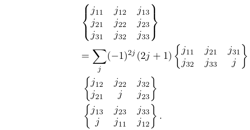
1: 34.6 Definition: $\mathit{9}j$ Symbol

§34.6 Definition: $\mathit{9}j$ Symbol

►The $\mathit{9}j$ symbol may be defined either in terms of $\mathit{3}j$ symbols or equivalently in terms of $\mathit{6}j$ symbols: ►

34.6.1

ⓘ

Defines:

: $\mathit{9}j$ symbol

Symbols:

: $\mathit{3}j$ symbol, $j,j_r$: non-negative integers or non-negative integers plus one half., $r$: nonnegative integer and $s$: integer

Permalink:

http://dlmf.nist.gov/34.6.E1

Encodings:

pMML, png, TeX

See also:

Annotations for §34.6 and Ch.34

►

34.6.2

ⓘ

Symbols:

: $\mathit{9}j$ symbol, : $\mathit{6}j$ symbol and $j,j_r$: non-negative integers or non-negative integers plus one half.

Referenced by:

§34.13

Permalink:

http://dlmf.nist.gov/34.6.E2

Encodings:

pMML, png, TeX

See also:

Annotations for §34.6 and Ch.34

►The $\mathit{9}j$ symbol may also be written as a finite triple sum equivalent to a terminating generalized hypergeometric series of three variables with unit arguments. …

2: 19.2 Definitions

… ►The principal values of $K\left(k\right)$ and $E\left(k\right)$ are even functions. … ►

§19.2(iv) A Related Function: $R_C(x,y)$

… ►Formulas involving $\mathrm{\Pi }(\varphi ,{\alpha }^2,k)$ that are customarily different for circular cases, ordinary hyperbolic cases, and (hyperbolic) Cauchy principal values, are united in a single formula by using $R_C(x,y)$. … ►When $x$ and $y$ are positive, $R_C(x,y)$ is an inverse circular function if and an inverse hyperbolic function (or logarithm) if $x>y$: …For the special cases of $R_C(x,x)$ and $R_C(0,y)$ see (19.6.15). …

3: Bibliography H

… ►

Solving Ordinary Differential Equations. I. Nonstiff Problems. 2nd edition, Springer Series in Computational Mathematics, Vol. 8, Springer-Verlag, Berlin.

ⓘ

Notes:

A reprinting with corrections appeared in 2000.

External Links:

ISBN 3-540-56670-8, MathReview, ZentralBlatt

Referenced by:

§3.7(v), §3.7(i).

Encodings:

BibTeX

… ►

Lamé polynomials of large order. SIAM J. Math. Anal. 8 (5), pp. 800–842.

ⓘ

External Links:

Document, MathReview (F. M. Arscott), ZentralBlatt

Referenced by:

§29.16.

Encodings:

BibTeX

… ►

Calculation of Coulomb wave functions for high energies. Phys. Rev. 54 (8), pp. 627–628.

ⓘ

External Links:

Document

Referenced by:

§33.7.

Encodings:

BibTeX

… ►

On congruences involving Bernoulli numbers and irregular primes. II. Rep. Fac. Sci. Technol. Meijo Univ. 31, pp. 1–8.

ⓘ

External Links:

ZentralBlatt

Referenced by:

§24.15(iii).

Encodings:

BibTeX

… ►

Coulomb Wave Functions. In Handbuch der Physik, Bd. 41/1, S. Flügge (Ed.), pp. 408–465.

ⓘ

External Links:

MathReview (G. Källén)

Referenced by:

§33.2(iii), §33.23(vii), §33.23(vii), §33.24, §33.5(ii), §33.7, Ch.33.

Encodings:

BibTeX

…

4: 3.4 Differentiation

… ►The $B_k^n$ are the differentiated Lagrangian interpolation coefficients: …where $A_k^n$ is as in (3.3.10). … ►

$$B_2^7=-\frac{1}{240}(72+36t-267t^2-80t^3+90t^4+12t^5-7t^6),$$

… ►where $C$ is a simple closed contour described in the positive rotational sense such that $C$ and its interior lie in the domain of analyticity of $f$, and $x_0$ is interior to $C$. Taking $C$ to be a circle of radius $r$ centered at $x_0$, we obtain …

5: 24.2 Definitions and Generating Functions

… ►

$B_{2n+1}=0$ ,

… ►

Table 24.2.3: Bernoulli numbers $B_n=N/D$.

► ►►►

$n$	$N$	$D$	$B_n$
…
$8$	$-1$	$30$	$-\mathrm{3.33333\hspace{0.33em}3333}$	$\mathrm{\times 10⁻²}$
…

►

►

Table 24.2.4: Euler numbers $E_n$.

► ►►►

$n$	$E_n$
…
$8$	$1385$
…

►

►

Table 24.2.5: Coefficients $b_{n,k}$ of the Bernoulli polynomials $B_n\left(x\right)={\sum }_{k=0}^n{b}_{n,k}{x}^k$.

► ►►►

	$k$
$n$	$0$	$1$	$2$	$3$	$4$	$5$	$6$	$7$	$8$	$9$	$10$	$11$	$12$	$13$	$14$	$15$
…

►

►

Table 24.2.6: Coefficients $e_{n,k}$ of the Euler polynomials $E_n\left(x\right)={\sum }_{k=0}^n{e}_{n,k}{x}^k$.

► ►►►

	$k$
$n$	$0$	$1$	$2$	$3$	$4$	$5$	$6$	$7$	$8$	$9$	$10$	$11$	$12$	$13$	$14$	$15$
…

►

6: 27.2 Functions

… ►

27.2.9 $$d\left(n\right)=\sum _{d|n}1$$

ⓘ

Symbols:

$d_k\left(n\right)$: divisor function, $d$: positive integer and $n$: positive integer

A&S Ref:

24.3.3 I.A

Permalink:

http://dlmf.nist.gov/27.2.E9

Encodings:

pMML, png, TeX

See also:

Annotations for §27.2(i), §27.2 and Ch.27

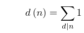
… ►It is the special case $k=2$ of the function $d_k\left(n\right)$ that counts the number of ways of expressing $n$ as the product of $k$ factors, with the order of factors taken into account. …Note that ${\sigma }_0\left(n\right)=d\left(n\right)$. … ►Table 27.2.2 tabulates the Euler totient function $\varphi \left(n\right)$, the divisor function $d\left(n\right)$ ($={\sigma }_0(n)$), and the sum of the divisors $\sigma (n)$ ($={\sigma }_1(n)$), for $n=1(1)52$. … ►

Table 27.2.2: Functions related to division.

► ►►►

$n$	$\varphi \left(n\right)$	$d\left(n\right)$	$\sigma \left(n\right)$	$n$	$\varphi \left(n\right)$	$d\left(n\right)$	$\sigma \left(n\right)$	$n$	$\varphi \left(n\right)$	$d\left(n\right)$	$\sigma \left(n\right)$	$n$	$\varphi \left(n\right)$	$d\left(n\right)$	$\sigma \left(n\right)$
1	1	1	1	14	6	4	24	27	18	4	40	40	16	8	90
…

►

7: 26.6 Other Lattice Path Numbers

… ►

Delannoy Number $D(m,n)$

► $D(m,n)$ is the number of paths from $(0,0)$ to $(m,n)$ that are composed of directed line segments of the form $(1,0)$, $(0,1)$, or $(1,1)$. … ►

Table 26.6.1: Delannoy numbers $D(m,n)$.

► ►►►

$m$	$n$
	0	1	2	3	4	5	6	7	8	9	10
…

►

… ►

Table 26.6.2: Motzkin numbers $M(n)$.

► ►►►

$n$	$M(n)$	$n$	$M(n)$	$n$	$M(n)$	$n$	$M(n)$	$n$	$M(n)$
0	1	4	9	8	323	12	15511	16	8 53467
…

►

… ►

Table 26.6.4: Schröder numbers $r(n)$.

► ►►►

$n$	$r(n)$	$n$	$r(n)$	$n$	$r(n)$	$n$	$r(n)$	$n$	$r(n)$
$0$	$1$	$4$	$90$	$8$	$41586$	$12$	$\mathrm{272\hspace{0.33em}97738}$	$16$	$\mathrm{2\hspace{0.33em}09271\hspace{0.33em}56706}$
…

►

…

8: 8 Incomplete Gamma and Related
Functions

Chapter 8 Incomplete Gamma and Related Functions

…

9: 1.12 Continued Fractions

… ► $C_n$ is called the $n$th approximant or convergent to $C$ . … ►Define … ►A contraction of a continued fraction $C$ is a continued fraction $C^{\prime }$ whose convergents $\{C_n^{\prime }\}$ form a subsequence of the convergents $\{C_n\}$ of $C$. Conversely, $C$ is called an extension of $C^{\prime }$. … ►Then the convergents $C_n$ satisfy …

10: Bibliography

… ►

Tables of $\ln \mathrm{\Gamma }(z)$ for Complex Argument. Pergamon Press, New York.

ⓘ

External Links:

ZentralBlatt

Referenced by:

§5.22(iii).

Encodings:

BibTeX

… ►

Supplement to a paper “On the intensity of light in the neighbourhood of a caustic”. Trans. Camb. Phil. Soc. 8, pp. 595–599.

ⓘ

Referenced by:

§9.16.

Encodings:

BibTeX

… ►

Frequency response characteristics of the multiport planar elliptic patch. IEEE Trans. Microwave Theory Tech. 40 (8), pp. 1726–1730.

ⓘ

External Links:

Document

Referenced by:

6th item.

Encodings:

BibTeX

… ►

Algorithm 588. Fast Hankel transforms using related and lagged convolutions. ACM Trans. Math. Software 8 (4), pp. 369–370.

ⓘ

Notes:

Single-precision Fortran, maximum accuracy 8S.

External Links:

ISSN 0098-3500, Document, GAMS (module 588; package TOMS)

Referenced by:

2nd item.

Encodings:

BibTeX

… ►

Chiral-symmetry breaking in QCD. I. The infrared domain. Phys. Rev. D (3) 37 (8), pp. 2290–2295.

ⓘ

External Links:

ISSN 0556-2821, Document, MathReview

Referenced by:

§15.18.

Encodings:

BibTeX

…