About the Project

%E5%8D%9A%E5%BD%A9%E6%8E%A8%E5%B9%BF%E8%AF%9D%E6%9C%AF,%E5%8D%9A%E5%BD%A9%E6%8E%A8%E5%B9%BF%E6%B8%A0%E9%81%93,%E5%8D%9A%E5%BD%A9%E5%BC%95%E6%B5%81%E6%96%B9%E5%BC%8F,%E3%80%90%E6%89%93%E5%BC%80%E7%BD%91%E5%9D%80%E2%88%B633kk88.com%E3%80%91%E5%8D%9A%E5%BD%A9%E6%8E%A8%E5%B9%BF%E6%8A%80%E5%B7%A7,%E5%8D%9A%E5%BD%A9seo%E6%8E%A8%E5%B9%BF%E6%B8%A0%E9%81%93,%E5%8D%9A%E5%BD%A9%E5%BC%95%E6%B5%81%E6%8A%80%E5%B7%A7,%E5%8D%9A%E5%BD%A9%E5%85%AC%E5%8F%B8%E6%8E%A8%E5%B9%BF%E6%96%B9%E6%B3%95,%E5%8D%9A%E5%BD%A9%E5%AE%A2%E6%88%B7%E8%AF%9D%E6%9C%AF,%E3%80%90%E5%8D%9A%E5%BD%A9%E5%9C%B0%E5%9D%80%E2%88%B633kk88.com%E3%80%91

AdvancedHelp

Did you mean %E5%8D%9A%E5%BD%A9%E6%8E%A8%E5%B9%BF%E8%AF%9D%E6%9C%AF,%E5%8D%9A%E5%BD%A9%E6%8E%A8%E5%B9%BF%E6%B8%A0%E9%81%93,%E5%8D%9A%E5%BD%A9%E5%BC%95%E6%B5%81%E6%96%B9%E5%BC%8F,%E3%80%90%E6%89%93%E5%BC%80%E7%BD%91%E5%9D%80%E2%88%gcn.com%E3%80%91%E5%8D%9A%E5%BD%A9%E6%8E%A8%E5%B9%BF%E6%8A%80%E5%B7%A7,%E5%8D%9A%E5%BD%base%E6%8E%A8%E5%B9%BF%E6%B8%A0%E9%81%93,%E5%8D%9A%E5%BD%A9%E5%BC%95%E6%B5%81%E6%8A%80%E5%B7%A7,%E5%8D%9A%E5%BD%A9%E5%85%AC%E5%8F%B8%E6%8E%A8%E5%B9%BF%E6%96%B9%E6%B3%95,%E5%8D%9A%E5%BD%A9%E5%AE%A2%E6%88%B7%E8%AF%9D%E6%9C%AF,%E3%80%90%E5%8D%9A%E5%BD%A9%E5%9C%B0%E5%9D%80%E2%88%gcn.com%E3%80%91 ?

(0.062 seconds)

1—10 of 603 matching pages
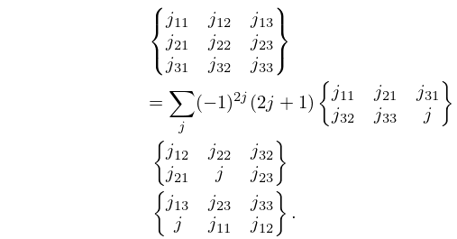
1: 34.6 Definition: 9 ⁒ j Symbol
§34.6 Definition: 9 ⁒ j Symbol
β–ΊThe 9 ⁒ j symbol may be defined either in terms of 3 ⁒ j symbols or equivalently in terms of 6 ⁒ j symbols: β–Ί
34.6.1 { j 11 j 12 j 13 j 21 j 22 j 23 j 31 j 32 j 33 } = all  ⁒ m r ⁒ s ( j 11 j 12 j 13 m 11 m 12 m 13 ) ⁒ ( j 21 j 22 j 23 m 21 m 22 m 23 ) ⁒ ( j 31 j 32 j 33 m 31 m 32 m 33 ) ⁒ ( j 11 j 21 j 31 m 11 m 21 m 31 ) ⁒ ( j 12 j 22 j 32 m 12 m 22 m 32 ) ⁒ ( j 13 j 23 j 33 m 13 m 23 m 33 ) ,
β–Ί
34.6.2 { j 11 j 12 j 13 j 21 j 22 j 23 j 31 j 32 j 33 } = j ( 1 ) 2 ⁒ j ⁒ ( 2 ⁒ j + 1 ) ⁒ { j 11 j 21 j 31 j 32 j 33 j } ⁒ { j 12 j 22 j 32 j 21 j j 23 } ⁒ { j 13 j 23 j 33 j j 11 j 12 } .
β–ΊThe 9 ⁒ j symbol may also be written as a finite triple sum equivalent to a terminating generalized hypergeometric series of three variables with unit arguments. …
2: 26.10 Integer Partitions: Other Restrictions
β–Ί p ⁑ ( π’Ÿ , n ) denotes the number of partitions of n into distinct parts. p m ⁑ ( π’Ÿ , n ) denotes the number of partitions of n into at most m distinct parts. … β–Ί
Table 26.10.1: Partitions restricted by difference conditions, or equivalently with parts from A j , k .
β–Ί β–Ίβ–Ίβ–Ί
p ⁑ ( π’Ÿ , n ) p ⁑ ( π’Ÿ ⁒ 2 , n ) p ⁑ ( π’Ÿ ⁒ 2 , T , n ) p ⁑ ( π’Ÿ ⁒ 3 , n )
9 8 5 3 3
β–Ί
β–ΊNote that p ⁑ ( π’Ÿ ⁒ 3 , n ) p ⁑ ( π’Ÿ ⁒ 3 , n ) , with strict inequality for n 9 . It is known that for k > 3 , p ⁑ ( π’Ÿ ⁒ k , n ) p ⁑ ( A 1 , k + 3 , n ) , with strict inequality for n sufficiently large, provided that k = 2 m 1 , m = 3 , 4 , 5 , or k 32 ; see Yee (2004). …
3: 26.6 Other Lattice Path Numbers
β–Ί
Delannoy Number D ⁑ ( m , n )
β–Ί D ⁑ ( m , n ) is the number of paths from ( 0 , 0 ) to ( m , n ) that are composed of directed line segments of the form ( 1 , 0 ) , ( 0 , 1 ) , or ( 1 , 1 ) . … β–Ί
Table 26.6.1: Delannoy numbers D ⁑ ( m , n ) .
β–Ί β–Ίβ–Ίβ–Ί
m n
0 1 2 3 4 5 6 7 8 9 10
β–Ί
β–Ί
Table 26.6.2: Motzkin numbers M ⁑ ( n ) .
β–Ί β–Ίβ–Ίβ–Ί
n M ⁑ ( n ) n M ⁑ ( n ) n M ⁑ ( n ) n M ⁑ ( n ) n M ⁑ ( n )
0 1 4 9 8 323 12 15511 16 8 53467
β–Ί
β–Ί
Table 26.6.3: Narayana numbers N ⁑ ( n , k ) .
β–Ί β–Ίβ–Ίβ–Ί
n k
0 1 2 3 4 5 6 7 8 9 10
β–Ί
4: 1.11 Zeros of Polynomials
β–ΊSet z = w 1 3 ⁒ a to reduce f ⁑ ( z ) = z 3 + a ⁒ z 2 + b ⁒ z + c to g ⁑ ( w ) = w 3 + p ⁒ w + q , with p = ( 3 ⁒ b a 2 ) / 3 , q = ( 2 ⁒ a 3 9 ⁒ a ⁒ b + 27 ⁒ c ) / 27 . … β–Ί f ⁑ ( z ) = z 3 6 ⁒ z 2 + 6 ⁒ z 2 , g ⁑ ( w ) = w 3 6 ⁒ w 6 , A = 3 ⁒ 4 3 , B = 3 ⁒ 2 3 . … β–ΊResolvent cubic is z 3 + 12 ⁒ z 2 + 20 ⁒ z + 9 = 0 with roots ΞΈ 1 = 1 , ΞΈ 2 = 1 2 ⁒ ( 11 + 85 ) , ΞΈ 3 = 1 2 ⁒ ( 11 85 ) , and ΞΈ 1 = 1 , ΞΈ 2 = 1 2 ⁒ ( 17 + 5 ) , ΞΈ 3 = 1 2 ⁒ ( 17 5 ) . … β–ΊLet … β–ΊThen f ⁑ ( z ) , with a n 0 , is stable iff a 0 0 ; D 2 ⁒ k > 0 , k = 1 , , 1 2 ⁒ n ; sign ⁑ D 2 ⁒ k + 1 = sign ⁑ a 0 , k = 0 , 1 , , 1 2 ⁒ n 1 2 .
5: 3.3 Interpolation
β–ΊIf f is analytic in a simply-connected domain D 1.13(i)), then for z D , …where C is a simple closed contour in D described in the positive rotational sense and enclosing the points z , z 1 , z 2 , , z n . … β–ΊIf f is analytic in a simply-connected domain D , then for z D , …where Ο‰ n + 1 ⁑ ( ΞΆ ) is given by (3.3.3), and C is a simple closed contour in D described in the positive rotational sense and enclosing z 0 , z 1 , , z n . … β–ΊThen by using x 3 in Newton’s interpolation formula, evaluating [ x 0 , x 1 , x 2 , x 3 ] ⁑ f = 0.26608 28233 and recomputing f ⁒ ( x ) , another application of Newton’s rule with starting value x 3 gives the approximation x = 2.33810 7373 , with 8 correct digits. …
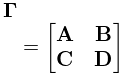
6: 21.5 Modular Transformations
β–ΊLet 𝐀 , 𝐁 , 𝐂 , and 𝐃 be g × g matrices with integer elements such that β–Ί
21.5.1 πšͺ = [ 𝐀 𝐁 𝐂 𝐃 ]
β–ΊHere ΞΎ ⁑ ( πšͺ ) is an eighth root of unity, that is, ( ΞΎ ⁑ ( πšͺ ) ) 8 = 1 . … β–Ί( 𝐀 invertible with integer elements.) …For a g × g matrix 𝐀 we define diag ⁒ 𝐀 , as a column vector with the diagonal entries as elements. …
7: 27.2 Functions
β–ΊIt is the special case k = 2 of the function d k ⁑ ( n ) that counts the number of ways of expressing n as the product of k factors, with the order of factors taken into account. …Note that Οƒ 0 ⁑ ( n ) = d ⁑ ( n ) . … β–ΊTable 27.2.2 tabulates the Euler totient function Ο• ⁑ ( n ) , the divisor function d ⁑ ( n ) ( = Οƒ 0 ⁑ ( n ) ), and the sum of the divisors Οƒ ⁑ ( n ) ( = Οƒ 1 ⁑ ( n ) ), for n = 1 ⁒ ( 1 ) ⁒ 52 . … β–Ί
Table 27.2.2: Functions related to division.
β–Ί β–Ίβ–Ίβ–Ίβ–Ί
n Ο• ⁑ ( n ) d ⁑ ( n ) Οƒ ⁑ ( n ) n Ο• ⁑ ( n ) d ⁑ ( n ) Οƒ ⁑ ( n ) n Ο• ⁑ ( n ) d ⁑ ( n ) Οƒ ⁑ ( n ) n Ο• ⁑ ( n ) d ⁑ ( n ) Οƒ ⁑ ( n )
3 2 2 4 16 8 5 31 29 28 2 30 42 12 8 96
11 10 2 12 24 8 8 60 37 36 2 38 50 20 6 93
β–Ί
8: 8 Incomplete Gamma and Related
Functions
Chapter 8 Incomplete Gamma and Related Functions
9: 28.25 Asymptotic Expansions for Large ⁑ z
β–Ί
28.25.1 M Ξ½ ( 3 , 4 ) ⁑ ( z , h ) e ± i ⁒ ( 2 ⁒ h ⁒ cosh ⁑ z ( 1 2 ⁒ Ξ½ + 1 4 ) ⁒ Ο€ ) ( Ο€ ⁒ h ⁒ ( cosh ⁑ z + 1 ) ) 1 2 ⁒ m = 0 D m ± ( βˆ“ 4 ⁒ i ⁒ h ⁒ ( cosh ⁑ z + 1 ) ) m ,
β–Ί
D 1 ± = 0 ,
β–Ί
D 0 ± = 1 ,
β–Ί
28.25.3 ( m + 1 ) ⁒ D m + 1 ± + ( ( m + 1 2 ) 2 ± ( m + 1 4 ) ⁒ 8 ⁒ i ⁒ h + 2 ⁒ h 2 a ) ⁒ D m ± ± ( m 1 2 ) ⁒ ( 8 ⁒ i ⁒ h ⁒ m ) ⁒ D m 1 ± = 0 , m 0 .
10: 28.8 Asymptotic Expansions for Large q
β–Ί
28.8.1 a m ⁑ ( h 2 ) b m + 1 ⁑ ( h 2 ) } 2 ⁒ h 2 + 2 ⁒ s ⁒ h 1 8 ⁒ ( s 2 + 1 ) 1 2 7 ⁒ h ⁒ ( s 3 + 3 ⁒ s ) 1 2 12 ⁒ h 2 ⁒ ( 5 ⁒ s 4 + 34 ⁒ s 2 + 9 ) 1 2 17 ⁒ h 3 ⁒ ( 33 ⁒ s 5 + 410 ⁒ s 3 + 405 ⁒ s ) 1 2 20 ⁒ h 4 ⁒ ( 63 ⁒ s 6 + 1260 ⁒ s 4 + 2943 ⁒ s 2 + 486 ) 1 2 25 ⁒ h 5 ⁒ ( 527 ⁒ s 7 + 15617 ⁒ s 5 + 69001 ⁒ s 3 + 41607 ⁒ s ) + β‹― .
β–ΊAlso let ΞΎ = 2 ⁒ h ⁒ cos ⁑ x and D m ⁑ ( ΞΎ ) = e ΞΎ 2 / 4 ⁒ 𝐻𝑒 m ⁑ ( ΞΎ ) 18.3). … β–Ί
28.8.4 U m ⁑ ( ΞΎ ) D m ⁑ ( ΞΎ ) 1 2 6 ⁒ h ⁒ ( D m + 4 ⁑ ( ΞΎ ) 4 ! ⁒ ( m 4 ) ⁒ D m 4 ⁑ ( ΞΎ ) ) + 1 2 13 ⁒ h 2 ⁒ ( D m + 8 ⁑ ( ΞΎ ) 2 5 ⁒ ( m + 2 ) ⁒ D m + 4 ⁑ ( ΞΎ ) + 4 ! ⁒  2 5 ⁒ ( m 1 ) ⁒ ( m 4 ) ⁒ D m 4 ⁑ ( ΞΎ ) + 8 ! ⁒ ( m 8 ) ⁒ D m 8 ⁑ ( ΞΎ ) ) + β‹― ,
β–Ί
28.8.5 V m ⁑ ( ΞΎ ) 1 2 4 ⁒ h ⁒ ( D m + 2 ⁑ ( ΞΎ ) m ⁒ ( m 1 ) ⁒ D m 2 ⁑ ( ΞΎ ) ) + 1 2 10 ⁒ h 2 ⁒ ( D m + 6 ⁑ ( ΞΎ ) + ( m 2 25 ⁒ m 36 ) ⁒ D m + 2 ⁑ ( ΞΎ ) m ⁒ ( m 1 ) ⁒ ( m 2 + 27 ⁒ m 10 ) ⁒ D m 2 ⁑ ( ΞΎ ) 6 ! ⁒ ( m 6 ) ⁒ D m 6 ⁑ ( ΞΎ ) ) + β‹― ,
β–Ί
28.8.6 C ^ m ( Ο€ ⁒ h 2 ⁒ ( m ! ) 2 ) 1 / 4 ⁒ ( 1 + 2 ⁒ m + 1 8 ⁒ h + m 4 + 2 ⁒ m 3 + 263 ⁒ m 2 + 262 ⁒ m + 108 2048 ⁒ h 2 + β‹― ) 1 / 2 ,