%E5%8D%9A%E5%BD%A9%E5%B9%B3%E5%8F%B0%E5%A4%A7%E5%85%A8,%E5%8D%9A%E5%BD%A9%E5%B9%B3%E5%8F%B0%E6%8E%92%E5%90%8D,%E7%BD%91%E4%B8%8A%E5%8D%9A%E5%BD%A9%E5%85%AC%E5%8F%B8,%E3%80%90%E5%8D%9A%E5%BD%A9%E7%BD%91%E5%9D%80%E2%88%B6789yule.com%E3%80%91%E5%85%A8%E7%90%83%E6%9C%80%E5%A4%A7%E7%9A%84%E5%8D%9A%E5%BD%A9%E5%B9%B3%E5%8F%B0,%E6%AD%A3%E8%A7%84%E5%8D%9A%E5%BD%A9%E5%B9%B3%E5%8F%B0%E6%8E%A8%E8%8D%90,%E4%BD%93%E8%82%B2%E5%8D%9A%E5%BD%A9%E5%85%AC%E5%8F%B8,%E4%BD%93%E8%82%B2%E5%8D%9A%E5%BD%A9%E5%B9%B3%E5%8F%B0%E6%8E%92%E5%90%8D%E3%80%90%E7%9C%9F%E4%BA%BA%E5%8D%9A%E5%BD%A9%E5%A4%A7%E5%8E%85%E2%88%B6789yule.com%E3%80%91

SearchAdvancedHelp

Did you mean %E5%8D%9A%E5%BD%A9%E5%B9%B3%E5%8F%B0%E5%A4%A7%E5%85%A8,%E5%8D%9A%E5%BD%A9%E5%B9%B3%E5%8F%B0%E6%8E%92%E5%90%8D,%E7%BD%91%E4%B8%8A%E5%8D%9A%E5%BD%A9%E5%85%AC%E5%8F%B8,%E3%80%90%E5%8D%9A%E5%BD%A9%E7%BD%91%E5%9D%80%E2%88%caniuse.com%E3%80%91%E5%85%A8%E7%90%83%E6%9C%80%E5%A4%A7%E7%9A%84%E5%8D%9A%E5%BD%A9%E5%B9%B3%E5%8F%B0,%E6%AD%A3%E8%A7%84%E5%8D%9A%E5%BD%A9%E5%B9%B3%E5%8F%B0%E6%8E%A8%E8%8D%90,%E4%BD%93%E8%82%B2%E5%8D%9A%E5%BD%A9%E5%85%AC%E5%8F%B8,%E4%BD%93%E8%82%B2%E5%8D%9A%E5%BD%A9%E5%B9%B3%E5%8F%B0%E6%8E%92%E5%90%8D%E3%80%90%E7%9C%9F%E4%BA%BA%E5%8D%9A%E5%BD%A9%E5%A4%A7%E5%8E%85%E2%88%caniuse.com%E3%80%91 ?

(0.085 seconds)

1—10 of 661 matching pages

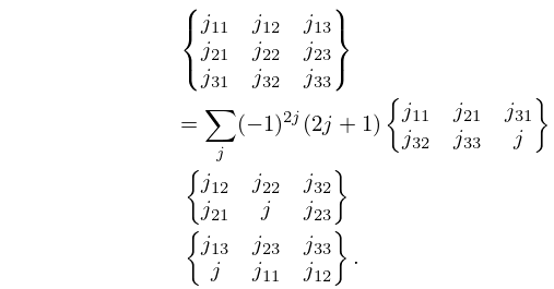
1: 34.6 Definition: $\mathit{9}j$ Symbol

§34.6 Definition: $\mathit{9}j$ Symbol

►The $\mathit{9}j$ symbol may be defined either in terms of $\mathit{3}j$ symbols or equivalently in terms of $\mathit{6}j$ symbols: ►

34.6.1

ⓘ

Defines:

: $\mathit{9}j$ symbol

Symbols:

: $\mathit{3}j$ symbol, $j,j_r$: non-negative integers or non-negative integers plus one half., $r$: nonnegative integer and $s$: integer

Permalink:

http://dlmf.nist.gov/34.6.E1

Encodings:

pMML, png, TeX

See also:

Annotations for §34.6 and Ch.34

►

34.6.2

ⓘ

Symbols:

: $\mathit{9}j$ symbol, : $\mathit{6}j$ symbol and $j,j_r$: non-negative integers or non-negative integers plus one half.

Referenced by:

§34.13

Permalink:

http://dlmf.nist.gov/34.6.E2

Encodings:

pMML, png, TeX

See also:

Annotations for §34.6 and Ch.34

►The $\mathit{9}j$ symbol may also be written as a finite triple sum equivalent to a terminating generalized hypergeometric series of three variables with unit arguments. …

2: 26.10 Integer Partitions: Other Restrictions

… ► $p(𝒟,n)$ denotes the number of partitions of $n$ into distinct parts. $p_m(𝒟,n)$ denotes the number of partitions of $n$ into at most $m$ distinct parts. $p(𝒟k,n)$ denotes the number of partitions of $n$ into parts with difference at least $k$. … ►Note that $p({𝒟}^{\prime }3,n)\le p(𝒟3,n)$, with strict inequality for $n\ge 9$. It is known that for $k>3$, $p(𝒟k,n)\ge p(\in A_{1,k+3},n)$, with strict inequality for $n$ sufficiently large, provided that $k=2^m-1,m=3,4,5$, or $k\ge 32$; see Yee (2004). …

3: 26.6 Other Lattice Path Numbers

… ►

Delannoy Number $D(m,n)$

► $D(m,n)$ is the number of paths from $(0,0)$ to $(m,n)$ that are composed of directed line segments of the form $(1,0)$, $(0,1)$, or $(1,1)$. … ►

Table 26.6.1: Delannoy numbers $D(m,n)$.

► ►►

$m$	$n$
	…

►

… ►

Table 26.6.2: Motzkin numbers $M(n)$.

► ►►►

$n$	$M(n)$	$n$	$M(n)$	$n$	$M(n)$	$n$	$M(n)$	$n$	$M(n)$
0	1	4	9	8	323	12	15511	16	8 53467
…

►

… ►

26.6.10 $$D(m,n)=D(m,n-1)+D(m-1,n)+D(m-1,n-1),$$ $m,n\ge 1$,

ⓘ

Symbols:

$m$: nonnegative integer, $n$: nonnegative integer and $D(m,n)$: Delannoy number

Referenced by:

§26.6(iii)

Permalink:

http://dlmf.nist.gov/26.6.E10

Encodings:

pMML, png, TeX

See also:

Annotations for §26.6(iii), §26.6 and Ch.26

…

4: 1.11 Zeros of Polynomials

… ►Set $z=w-\frac{1}{3}a$ to reduce $f(z)=z^3+a{z}^2+bz+c$ to $g(w)=w^3+pw+q$, with $p=(3b-a^2)/3$, $q=(2a^3-9ab+27c)/27$. … ► $f(z)=z^3-6z^2+6z-2$, $g(w)=w^3-6w-6$, $A=3\sqrt[3]{4}$, $B=3\sqrt[3]{2}$. … ►Resolvent cubic is $z^3+12z^2+20z+9=0$ with roots ${\theta }_1=-1$, ${\theta }_2=-\frac{1}{2}(11+\sqrt{85})$, ${\theta }_3=-\frac{1}{2}(11-\sqrt{85})$, and $\sqrt{-{\theta }_1}=1$, $\sqrt{-{\theta }_2}=\frac{1}{2}(\sqrt{17}+\sqrt{5})$, $\sqrt{-{\theta }_3}=\frac{1}{2}(\sqrt{17}-\sqrt{5})$. … ►Let … ►Then $f(z)$, with $a_n\ne 0$, is stable iff $a_0\ne 0$; $D_{2k}>0$, $k=1,\mathrm{\dots },\lfloor \frac{1}{2}n\rfloor$; $\mathrm{sign}{D}_{2k+1}=\mathrm{sign}{a}_0$, $k=0,1,\mathrm{\dots },\lfloor \frac{1}{2}n-\frac{1}{2}\rfloor$.

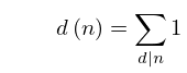
5: 27.2 Functions

… ►

27.2.9 $$d\left(n\right)=\sum _{d|n}1$$

ⓘ

Symbols:

$d_k\left(n\right)$: divisor function, $d$: positive integer and $n$: positive integer

A&S Ref:

24.3.3 I.A

Permalink:

http://dlmf.nist.gov/27.2.E9

Encodings:

pMML, png, TeX

See also:

Annotations for §27.2(i), §27.2 and Ch.27

… ►It is the special case $k=2$ of the function $d_k\left(n\right)$ that counts the number of ways of expressing $n$ as the product of $k$ factors, with the order of factors taken into account. …Note that ${\sigma }_0\left(n\right)=d\left(n\right)$. … ►Table 27.2.2 tabulates the Euler totient function $\varphi \left(n\right)$, the divisor function $d\left(n\right)$ ($={\sigma }_0(n)$), and the sum of the divisors $\sigma (n)$ ($={\sigma }_1(n)$), for $n=1(1)52$. … ►

Table 27.2.2: Functions related to division.

► ►►►

$n$	$\varphi \left(n\right)$	$d\left(n\right)$	$\sigma \left(n\right)$	$n$	$\varphi \left(n\right)$	$d\left(n\right)$	$\sigma \left(n\right)$	$n$	$\varphi \left(n\right)$	$d\left(n\right)$	$\sigma \left(n\right)$	$n$	$\varphi \left(n\right)$	$d\left(n\right)$	$\sigma \left(n\right)$
…
11	10	2	12	24	8	8	60	37	36	2	38	50	20	6	93
…

►

6: Bibliography H

… ►

Solving Ordinary Differential Equations. I. Nonstiff Problems. 2nd edition, Springer Series in Computational Mathematics, Vol. 8, Springer-Verlag, Berlin.

ⓘ

Notes:

A reprinting with corrections appeared in 2000.

External Links:

ISBN 3-540-56670-8, MathReview, ZentralBlatt

Referenced by:

§3.7(v), §3.7(i).

Encodings:

BibTeX

… ►

Lamé polynomials of large order. SIAM J. Math. Anal. 8 (5), pp. 800–842.

ⓘ

External Links:

Document, MathReview (F. M. Arscott), ZentralBlatt

Referenced by:

§29.16.

Encodings:

BibTeX

… ►

Calculation of Coulomb wave functions for high energies. Phys. Rev. 54 (8), pp. 627–628.

ⓘ

External Links:

Document

Referenced by:

§33.7.

Encodings:

BibTeX

… ►

On congruences involving Bernoulli numbers and irregular primes. II. Rep. Fac. Sci. Technol. Meijo Univ. 31, pp. 1–8.

ⓘ

External Links:

ZentralBlatt

Referenced by:

§24.15(iii).

Encodings:

BibTeX

… ►

Coulomb Wave Functions. In Handbuch der Physik, Bd. 41/1, S. Flügge (Ed.), pp. 408–465.

ⓘ

External Links:

MathReview (G. Källén)

Referenced by:

§33.2(iii), §33.23(vii), §33.23(vii), §33.24, §33.5(ii), §33.7, Ch.33.

Encodings:

BibTeX

…

7: 3.3 Interpolation

… ►If $f$ is analytic in a simply-connected domain $D$ (§1.13(i)), then for $z\in D$, …where $C$ is a simple closed contour in $D$ described in the positive rotational sense and enclosing the points $z,z_1,z_2,\mathrm{\dots },z_n$. … ►If $f$ is analytic in a simply-connected domain $D$, then for $z\in D$, …where ${\omega }_{n+1}(\zeta )$ is given by (3.3.3), and $C$ is a simple closed contour in $D$ described in the positive rotational sense and enclosing $z_0,z_1,\mathrm{\dots },z_n$. … ►Then by using $x_3$ in Newton’s interpolation formula, evaluating $\left[x_0,x_1,x_2,x_3\right]f=-\mathrm{0.26608\hspace{0.33em}28233}$ and recomputing $f^{\prime }(x)$, another application of Newton’s rule with starting value $x_3$ gives the approximation $x=\mathrm{2.33810\hspace{0.33em}7373}$, with 8 correct digits. …

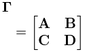
8: 21.5 Modular Transformations

… ►Let $𝐀$, $𝐁$, $𝐂$, and $𝐃$ be $g\times g$ matrices with integer elements such that ►

21.5.1

ⓘ

Defines:

Matrix $𝚪$ (locally)

Permalink:

http://dlmf.nist.gov/21.5.E1

Encodings:

pMML, png, TeX

See also:

Annotations for §21.5(i), §21.5 and Ch.21

… ►Here $\xi (𝚪)$ is an eighth root of unity, that is, ${(\xi (𝚪))}^8=1$. … ►($𝐀$ invertible with integer elements.) …For a $g\times g$ matrix $𝐀$ we define $\mathrm{diag}𝐀$, as a column vector with the diagonal entries as elements. …

9: 8 Incomplete Gamma and Related
Functions

Chapter 8 Incomplete Gamma and Related Functions

…

10: Bibliography

… ►

Tables of $\ln \mathrm{\Gamma }(z)$ for Complex Argument. Pergamon Press, New York.

ⓘ

External Links:

ZentralBlatt

Referenced by:

§5.22(iii).

Encodings:

BibTeX

… ►

Supplement to a paper “On the intensity of light in the neighbourhood of a caustic”. Trans. Camb. Phil. Soc. 8, pp. 595–599.

ⓘ

Referenced by:

§9.16.

Encodings:

BibTeX

… ►

Frequency response characteristics of the multiport planar elliptic patch. IEEE Trans. Microwave Theory Tech. 40 (8), pp. 1726–1730.

ⓘ

External Links:

Document

Referenced by:

6th item.

Encodings:

BibTeX

… ►

Algorithm 588. Fast Hankel transforms using related and lagged convolutions. ACM Trans. Math. Software 8 (4), pp. 369–370.

ⓘ

Notes:

Single-precision Fortran, maximum accuracy 8S.

External Links:

ISSN 0098-3500, Document, GAMS (module 588; package TOMS)

Referenced by:

2nd item.

Encodings:

BibTeX

… ►

Normal forms of functions near degenerate critical points, the Weyl groups $A_k,D_k,E_k$ and Lagrangian singularities. Funkcional. Anal. i Priložen. 6 (4), pp. 3–25 (Russian).

ⓘ

Notes:

In Russian. English translation: Functional Anal. Appl., 6(1973), pp. 254–272.

External Links:

MathReview (G. R. Belickii), ZentralBlatt

Referenced by:

§36.2(i).

Encodings:

BibTeX

…