Visit (-- RXLARA.COM --) pharmacy buy Femara over counter. Letrozole Femara 2.5mg pills price prescription online

SearchAdvancedHelp

Did you mean Visit (-- welcom --) pharmacy buy maria over counterpart. petropoule maria 2.5mg mills price prescription online ?

(0.010 seconds)

1—10 of 345 matching pages

1: 12.19 Tables

… ►

Abramowitz and Stegun (1964, Chapter 19) includes $U(a,x)$ and $V(a,x)$ for $\pm a=0(.1)1(.5)5$, $x=0(.1)5$, 5S; $W(a,\pm x)$ for $\pm a=0(.1)1(1)5$, $x=0(.1)5$, 4-5D or 4-5S.

… ►

Kireyeva and Karpov (1961) includes $D_p\left(x(1+\mathrm{i})\right)$ for $\pm x=0(.1)5$, $p=0(.1)2$, and $\pm x=5(.01)10$, $p=0(.5)2$, 7D.

►

Karpov and Čistova (1964) includes $D_p\left(x\right)$ for $p=-2(.1)0$, $\pm x=0(.01)5$; $p=-2(.05)0$, $\pm x=5(.01)10$, 6D.

… ►

Zhang and Jin (1996, pp. 455–473) includes $U(\pm n-\frac{1}{2},x)$, $V(\pm n-\frac{1}{2},x)$, $U(\pm \nu -\frac{1}{2},x)$, $V(\pm \nu -\frac{1}{2},x)$, and derivatives, $\nu =n+\frac{1}{2}$, $n=0(1)10(10)30$, $x=0.5,1,5,10,30,50$, 8S; $W(a,\pm x)$, $W(-a,\pm x)$, and derivatives, $a=h(1)5+h$, $x=0.5,1$ and $a=h(1)5+h$, $x=5$, $h=0,0.5$, 8S. Also, first zeros of $U(a,x)$, $V(a,x)$, and of derivatives, $a=-6(.5)-1$, 6D; first three zeros of $W(a,-x)$ and of derivative, $a=0(.5)4$, 6D; first three zeros of $W(-a,\pm x)$ and of derivative, $a=0.5(.5)5.5$, 6D; real and imaginary parts of $U(a,z)$, $a=-1.5(1)1.5$, $z=x+\mathrm{i}y$, $x=0.5,1,5,10$, $y=0(.5)10$, 8S.

…

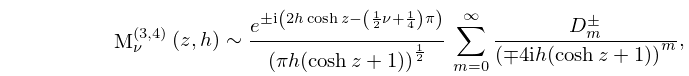
2: 11.8 Analogs to Kelvin Functions

§11.8 Analogs to Kelvin Functions

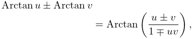
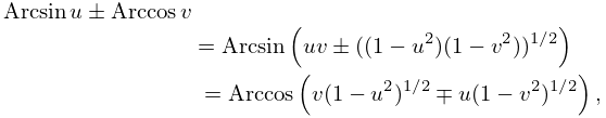
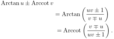
►For properties of Struve functions of argument $x{\mathrm{e}}^{\pm 3\pi \mathrm{i}/4}$ see McLachlan and Meyers (1936).

3: 4.16 Elementary Properties

… ►

Table 4.16.2: Trigonometric functions: quarter periods and change of sign.

► ►►►►►►

$x$	$-\theta$	$\frac{1}{2}\pi \pm \theta$	$\pi \pm \theta$	$\frac{3}{2}\pi \pm \theta$	$2\pi \pm \theta$
$\sin x$	$-\sin \theta$	$\cos \theta$	$\mp \sin \theta$	$-\cos \theta$	$\pm \sin \theta$
$\cos x$	$\cos \theta$	$\mp \sin \theta$	$-\cos \theta$	$\pm \sin \theta$	$\cos \theta$
$\tan x$	$-\tan \theta$	$\mp \cot \theta$	$\pm \tan \theta$	$\mp \cot \theta$	$\pm \tan \theta$
…
$\cot x$	$-\cot \theta$	$\mp \tan \theta$	$\pm \cot \theta$	$\mp \tan \theta$	$\pm \cot \theta$

►

…

4: 28.25 Asymptotic Expansions for Large $\mathrm{\Re }z$

… ►

28.25.1 $${\mathrm{M}}_{\nu }^{(3,4)}(z,h)\sim \frac{{\mathrm{e}}^{\pm \mathrm{i}\left(2h\cosh z-\left(\frac{1}{2}\nu +\frac{1}{4}\right)\pi \right)}}{{\left(\pi h(\cosh z+1)\right)}^{\frac{1}{2}}}\sum _{m=0}^{\mathrm{\infty }}\frac{D_m^{\pm }}{{\left(\mp 4\mathrm{i}h(\cosh z+1)\right)}^m},$$

ⓘ

Symbols:

$\sim$: Poincaré asymptotic expansion, $\pi$: the ratio of the circumference of a circle to its diameter, $\mathrm{e}$: base of natural logarithm, $\cosh z$: hyperbolic cosine function, $\mathrm{i}$: imaginary unit, ${\mathrm{M}}_{\nu }^{(j)}(z,h)$: modified Mathieu function, $m$: integer, $h$: parameter, $z$: complex variable, $\nu$: complex parameter and $D_m^{\pm }$: coefficients

A&S Ref:

20.9.1 (for 3 and for integer $\nu$) 20.9.3 (for 4 and for integer $\nu$)

Referenced by:

§28.25

Permalink:

http://dlmf.nist.gov/28.25.E1

Encodings:

pMML, png, TeX

See also:

Annotations for §28.25 and Ch.28

… ►

$D_{-1}^{\pm }=0,$

►

$D_0^{\pm }=1,$

… ►

28.25.3 $$(m+1)D_{m+1}^{\pm }+\left({(m+\frac{1}{2})}^2\pm (m+\frac{1}{4})8\mathrm{i}h+2h^2-a\right)D_m^{\pm }\pm (m-\frac{1}{2})\left(8\mathrm{i}hm\right)D_{m-1}^{\pm }=0,$$ $m\ge 0$.

ⓘ

Symbols:

$\mathrm{i}$: imaginary unit, $m$: integer, $h$: parameter, $a$: parameter and $D_m^{\pm }$: coefficients

A&S Ref:

20.9.2 (for $+$) 20.9.4 (for $-$)

Permalink:

http://dlmf.nist.gov/28.25.E3

Encodings:

pMML, png, TeX

See also:

Annotations for §28.25 and Ch.28

…

5: 4.13 Lambert $W$-Function

… ►The decreasing solution can be identified as $W_{\pm 1}\left(x\mp 0\mathrm{i}\right)$. …$W_0\left(z\right)$ is a single-valued analytic function on $ℂ\setminus (-\mathrm{\infty },-{\mathrm{e}}^{-1}]$, real-valued when $z>-{\mathrm{e}}^{-1}$, and has a square root branch point at $z=-{\mathrm{e}}^{-1}$. …The other branches $W_k\left(z\right)$ are single-valued analytic functions on $ℂ\setminus (-\mathrm{\infty },0]$, have a logarithmic branch point at $z=0$, and, in the case $k=\pm 1$, have a square root branch point at $z=-{\mathrm{e}}^{-1}\mp 0\mathrm{i}$ respectively. … ►and has several advantages over the Lambert $W$-function (see Lawrence et al. (2012)), and the tree $T$-function $T\left(z\right)=-W\left(-z\right)$, which is a solution of … ►where $t\ge 0$ for $W_0$, $t\le 0$ for $W_{\pm 1}$ on the relevant branch cuts, …

6: 36.7 Zeros

… ►

$$x_{m,n}^{\pm }=\sqrt{\frac{2}{-y_m}}\left(2n+\frac{1}{2}+{(-1)}^m\frac{1}{2}\pm \frac{1}{4}\right)\pi ,$$ $m=1,2,3,\mathrm{\dots }$, $n=0,\pm 1,\pm 2,\mathrm{\dots }$.

►

Table 36.7.1: Zeros of cusp diffraction catastrophe to 5D. …

► ►►►►►

Zeros $\left\{\genfrac{}{}{0.0pt}{}{x}{y}\right\}$ inside, and zeros $\left[\genfrac{}{}{0.0pt}{}{x}{y}\right]$ outside, the cusp $x^2=\frac{8}{27}{|y|}^3$.
$\left\{{\displaystyle \genfrac{}{}{0.0pt}{}{\pm 0.52768}{-4.37804}}\right\}$	$\left[{\displaystyle \genfrac{}{}{0.0pt}{}{\pm 2.35218}{-1.74360}}\right]$
$\left\{{\displaystyle \genfrac{}{}{0.0pt}{}{\pm 1.41101}{-5.55470}}\right\}$	$\left\{{\displaystyle \genfrac{}{}{0.0pt}{}{\pm 2.36094}{-5.52321}}\right\}$	$\left[{\displaystyle \genfrac{}{}{0.0pt}{}{\pm 4.42707}{-3.05791}}\right]$
…
$\left\{{\displaystyle \genfrac{}{}{0.0pt}{}{\pm 0.38488}{-8.31916}}\right\}$	$\left\{{\displaystyle \genfrac{}{}{0.0pt}{}{\pm 2.71193}{-8.22315}}\right\}$	$\left\{{\displaystyle \genfrac{}{}{0.0pt}{}{\pm 3.49286}{-8.20326}}\right\}$	$\left\{{\displaystyle \genfrac{}{}{0.0pt}{}{\pm 5.96669}{-7.85723}}\right\}$	$\left\{{\displaystyle \genfrac{}{}{0.0pt}{}{\pm 6.79538}{-7.80456}}\right\}$	$\left[{\displaystyle \genfrac{}{}{0.0pt}{}{\pm 9.17308}{-5.55831}}\right]$

►

… ►

$x_n=\pm {\left({\displaystyle \frac{8}{27}}\right)}^{1/2}{|y_n|}^{3/2}(1+{\xi }_n),$

…

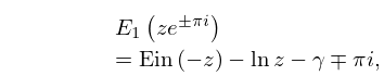
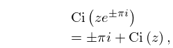
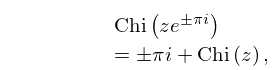
7: 6.4 Analytic Continuation

… ►

6.4.3 $$E_1\left(z{\mathrm{e}}^{\pm \pi \mathrm{i}}\right)=\mathrm{Ein}\left(-z\right)-\ln z-\gamma \mp \pi \mathrm{i},$$ $|\mathrm{ph}z|\le \pi$.

ⓘ

Symbols:

$\gamma$: Euler’s constant, $\pi$: the ratio of the circumference of a circle to its diameter, $\mathrm{Ein}\left(z\right)$: complementary exponential integral, $\mathrm{e}$: base of natural logarithm, $E_1\left(z\right)$: exponential integral, $\mathrm{i}$: imaginary unit, $\ln z$: principal branch of logarithm function, $\mathrm{ph}$: phase and $z$: complex variable

Referenced by:

§6.4

Permalink:

http://dlmf.nist.gov/6.4.E3

Encodings:

pMML, png, TeX

See also:

Annotations for §6.4 and Ch.6

… ►

6.4.4 $$\mathrm{Ci}\left(z{\mathrm{e}}^{\pm \pi \mathrm{i}}\right)=\pm \pi \mathrm{i}+\mathrm{Ci}\left(z\right),$$

ⓘ

Symbols:

$\pi$: the ratio of the circumference of a circle to its diameter, $\mathrm{Ci}\left(z\right)$: cosine integral, $\mathrm{e}$: base of natural logarithm, $\mathrm{i}$: imaginary unit and $z$: complex variable

Referenced by:

§6.4

Permalink:

http://dlmf.nist.gov/6.4.E4

Encodings:

pMML, png, TeX

See also:

Annotations for §6.4 and Ch.6

►

6.4.5 $$\mathrm{Chi}\left(z{\mathrm{e}}^{\pm \pi \mathrm{i}}\right)=\pm \pi \mathrm{i}+\mathrm{Chi}\left(z\right),$$

ⓘ

Symbols:

$\pi$: the ratio of the circumference of a circle to its diameter, $\mathrm{e}$: base of natural logarithm, $\mathrm{Chi}\left(z\right)$: hyperbolic cosine integral, $\mathrm{i}$: imaginary unit and $z$: complex variable

Referenced by:

§6.4

Permalink:

http://dlmf.nist.gov/6.4.E5

Encodings:

pMML, png, TeX

See also:

Annotations for §6.4 and Ch.6

►

6.4.6 $$\mathrm{f}\left(z{\mathrm{e}}^{\pm \pi \mathrm{i}}\right)=\pi {\mathrm{e}}^{\mp \mathrm{i}z}-\mathrm{f}\left(z\right),$$

ⓘ

Symbols:

$\pi$: the ratio of the circumference of a circle to its diameter, $\mathrm{e}$: base of natural logarithm, $\mathrm{i}$: imaginary unit, $\mathrm{f}\left(z\right)$: auxiliary function for sine and cosine integrals and $z$: complex variable

Referenced by:

§6.12(ii), §6.4

Permalink:

http://dlmf.nist.gov/6.4.E6

Encodings:

pMML, png, TeX

See also:

Annotations for §6.4 and Ch.6

►

6.4.7 $$\mathrm{g}\left(z{\mathrm{e}}^{\pm \pi \mathrm{i}}\right)=\mp \pi \mathrm{i}{\mathrm{e}}^{\mp \mathrm{i}z}+\mathrm{g}\left(z\right).$$

ⓘ

Symbols:

$\pi$: the ratio of the circumference of a circle to its diameter, $\mathrm{e}$: base of natural logarithm, $\mathrm{i}$: imaginary unit, $\mathrm{g}\left(z\right)$: auxiliary function for sine and cosine integrals and $z$: complex variable

Referenced by:

§6.12(ii), §6.4

Permalink:

http://dlmf.nist.gov/6.4.E7

Encodings:

pMML, png, TeX

See also:

Annotations for §6.4 and Ch.6

…

8: 26.15 Permutations: Matrix Notation

… ►where the sum is over and $n\ge h>\mathrm{\ell }\ge 1$. … ►For $(j,k)\in B$, $B\setminus [j,k]$ denotes $B$ after removal of all elements of the form $(j,t)$ or $(t,k)$, $t=1,2,\mathrm{\dots },n$. $B\setminus (j,k)$ denotes $B$ with the element $(j,k)$ removed. ►

26.15.5 $$R(x,B)=xR(x,B\setminus [j,k])+R(x,B\setminus (j,k)).$$

ⓘ

Symbols:

$[a,b]$: closed interval, $(a,b)$: open interval, $\setminus$: set subtraction, $x$: real variable, $j$: nonnegative integer, $k$: nonnegative integer, $B$: subset and $R(x,B)$: rook polynomial

Permalink:

http://dlmf.nist.gov/26.15.E5

Encodings:

pMML, png, TeX

See also:

Annotations for §26.15 and Ch.26

…

9: 33.8 Continued Fractions

… ►

33.8.2 $$\frac{H_{\mathrm{\ell }}^{\pm }{}_{}{}^{\prime }}{H_{\mathrm{\ell }}^{\pm }}=c\pm \frac{\mathrm{i}}{\rho }\frac{ab}{2(\rho -\eta \pm \mathrm{i})+}\frac{(a+1)(b+1)}{2(\rho -\eta \pm 2\mathrm{i})+}\mathrm{\cdots },$$

ⓘ

Symbols:

$\mathrm{i}$: imaginary unit, $H_{\mathrm{\ell }}^{\pm }(\eta ,\rho )$: irregular Coulomb radial functions, $\mathrm{\ell }$: nonnegative integer, $\rho$: nonnegative real variable, $\eta$: real parameter, $a$: coefficient, $b$: coefficient and $c$: coefficient

Referenced by:

§33.8

Permalink:

http://dlmf.nist.gov/33.8.E2

Encodings:

pMML, png, TeX

See also:

Annotations for §33.8 and Ch.33

… ►

$a=1+\mathrm{\ell }\pm \mathrm{i}\eta ,$

►

$b=-\mathrm{\ell }\pm \mathrm{i}\eta ,$

►

$c=\pm \mathrm{i}(1-(\eta /\rho )).$

… ►

$F_{\mathrm{\ell }}=\pm {(q^{-1}{(u-p)}^2+q)}^{-1/2},$

…

10: 4.24 Inverse Trigonometric Functions: Further Properties

… ►

4.24.13 $$\mathrm{Arcsin}u\pm \mathrm{Arcsin}v=\mathrm{Arcsin}\left(u{(1-v^2)}^{1/2}\pm v{(1-u^2)}^{1/2}\right),$$

ⓘ

Symbols:

$\mathrm{Arcsin}z$: general arcsine function

A&S Ref:

4.4.32

Permalink:

http://dlmf.nist.gov/4.24.E13

Encodings:

pMML, png, TeX

See also:

Annotations for §4.24(iii), §4.24 and Ch.4

►

4.24.14 $$\mathrm{Arccos}u\pm \mathrm{Arccos}v=\mathrm{Arccos}\left(uv\mp {((1-u^2)(1-v^2))}^{1/2}\right),$$

ⓘ

Symbols:

$\mathrm{Arccos}z$: general arccosine function

A&S Ref:

4.4.33

Permalink:

http://dlmf.nist.gov/4.24.E14

Encodings:

pMML, png, TeX

See also:

Annotations for §4.24(iii), §4.24 and Ch.4

►

4.24.15 $$\mathrm{Arctan}u\pm \mathrm{Arctan}v=\mathrm{Arctan}\left(\frac{u\pm v}{1\mp uv}\right),$$

ⓘ

Symbols:

$\mathrm{Arctan}z$: general arctangent function

A&S Ref:

4.4.34

Referenced by:

§4.45(i)

Permalink:

http://dlmf.nist.gov/4.24.E15

Encodings:

pMML, png, TeX

See also:

Annotations for §4.24(iii), §4.24 and Ch.4

►

4.24.16 $$\mathrm{Arcsin}u\pm \mathrm{Arccos}v=\mathrm{Arcsin}\left(uv\pm {((1-u^2)(1-v^2))}^{1/2}\right)=\mathrm{Arccos}\left(v{(1-u^2)}^{1/2}\mp u{(1-v^2)}^{1/2}\right),$$

ⓘ

Symbols:

$\mathrm{Arccos}z$: general arccosine function and $\mathrm{Arcsin}z$: general arcsine function

A&S Ref:

4.4.35

Permalink:

http://dlmf.nist.gov/4.24.E16

Encodings:

pMML, png, TeX

See also:

Annotations for §4.24(iii), §4.24 and Ch.4

►

4.24.17 $$\mathrm{Arctan}u\pm \mathrm{Arccot}v=\mathrm{Arctan}\left(\frac{uv\pm 1}{v\mp u}\right)=\mathrm{Arccot}\left(\frac{v\mp u}{uv\pm 1}\right).$$

ⓘ

Symbols:

$\mathrm{Arccot}z$: general arccotangent function and $\mathrm{Arctan}z$: general arctangent function

A&S Ref:

4.4.36

Permalink:

http://dlmf.nist.gov/4.24.E17

Encodings:

pMML, png, TeX

See also:

Annotations for §4.24(iii), §4.24 and Ch.4

…