Visit (-- RXLARA.COM --) pharmacy buy Caverta over counter. Sildenafil Citrate Caverta 50-100mg pills price prescription online r

SearchAdvancedHelp

Did you mean Visit (-- welcom --) pharmacy buy averag over counterpart. ident stratege averag 50-100mg mills price prescription online r ?

(0.011 seconds)

1—10 of 456 matching pages

1: 36.7 Zeros

… ►

$$x_{m,n}^{\pm }=\sqrt{\frac{2}{-y_m}}\left(2n+\frac{1}{2}+{(-1)}^m\frac{1}{2}\pm \frac{1}{4}\right)\pi ,$$ $m=1,2,3,\mathrm{\dots }$, $n=0,\pm 1,\pm 2,\mathrm{\dots }$.

►

Table 36.7.1: Zeros of cusp diffraction catastrophe to 5D. …

► ►►►►

Zeros $\left\{\genfrac{}{}{0.0pt}{}{x}{y}\right\}$ inside, and zeros $\left[\genfrac{}{}{0.0pt}{}{x}{y}\right]$ outside, the cusp $x^2=\frac{8}{27}{|y|}^3$.
…
$\left\{{\displaystyle \genfrac{}{}{0.0pt}{}{\pm 1.41101}{-5.55470}}\right\}$	$\left\{{\displaystyle \genfrac{}{}{0.0pt}{}{\pm 2.36094}{-5.52321}}\right\}$	$\left[{\displaystyle \genfrac{}{}{0.0pt}{}{\pm 4.42707}{-3.05791}}\right]$
…
$\left\{{\displaystyle \genfrac{}{}{0.0pt}{}{\pm 0.38488}{-8.31916}}\right\}$	$\left\{{\displaystyle \genfrac{}{}{0.0pt}{}{\pm 2.71193}{-8.22315}}\right\}$	$\left\{{\displaystyle \genfrac{}{}{0.0pt}{}{\pm 3.49286}{-8.20326}}\right\}$	$\left\{{\displaystyle \genfrac{}{}{0.0pt}{}{\pm 5.96669}{-7.85723}}\right\}$	$\left\{{\displaystyle \genfrac{}{}{0.0pt}{}{\pm 6.79538}{-7.80456}}\right\}$	$\left[{\displaystyle \genfrac{}{}{0.0pt}{}{\pm 9.17308}{-5.55831}}\right]$

►

… ►

$x_n=\pm {\left({\displaystyle \frac{8}{27}}\right)}^{1/2}{|y_n|}^{3/2}(1+{\xi }_n),$

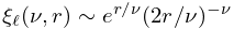
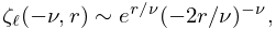
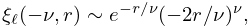
… ►There are also three sets of zero lines in the plane $z=0$ related by $2\pi /3$ rotation; these are zeros of (36.2.20), whose asymptotic form in polar coordinates $(x=r\cos \theta ,y=r\sin \theta )$ is given by …

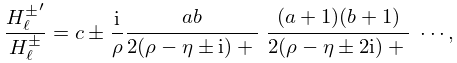
2: 33.8 Continued Fractions

… ►For $R$, $S$, and $T$ see (33.4.1). ►

33.8.2 $$\frac{H_{\mathrm{\ell }}^{\pm }{}_{}{}^{\prime }}{H_{\mathrm{\ell }}^{\pm }}=c\pm \frac{\mathrm{i}}{\rho }\frac{ab}{2(\rho -\eta \pm \mathrm{i})+}\frac{(a+1)(b+1)}{2(\rho -\eta \pm 2\mathrm{i})+}\mathrm{\cdots },$$

ⓘ

Symbols:

$\mathrm{i}$: imaginary unit, $H_{\mathrm{\ell }}^{\pm }(\eta ,\rho )$: irregular Coulomb radial functions, $\mathrm{\ell }$: nonnegative integer, $\rho$: nonnegative real variable, $\eta$: real parameter, $a$: coefficient, $b$: coefficient and $c$: coefficient

Referenced by:

§33.8

Permalink:

http://dlmf.nist.gov/33.8.E2

Encodings:

pMML, png, TeX

See also:

Annotations for §33.8 and Ch.33

… ►

$a=1+\mathrm{\ell }\pm \mathrm{i}\eta ,$

►

$b=-\mathrm{\ell }\pm \mathrm{i}\eta ,$

►

$c=\pm \mathrm{i}(1-(\eta /\rho )).$

…

3: 19.2 Definitions

… ►Let $s^2(t)$ be a cubic or quartic polynomial in $t$ with simple zeros, and let $r(s,t)$ be a rational function of $s$ and $t$ containing at least one odd power of $s$. … ►Assume $1-{\sin }^2\varphi \in ℂ\setminus (-\mathrm{\infty },0]$ and $1-k^2{\sin }^2\varphi \in ℂ\setminus (-\mathrm{\infty },0]$, except that one of them may be 0, and $1-{\alpha }^2{\sin }^2\varphi \in ℂ\setminus \{0\}$. … ►

§19.2(iv) A Related Function: $R_C(x,y)$

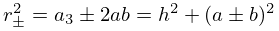
►Let $x\in ℂ\setminus (-\mathrm{\infty },0)$ and $y\in ℂ\setminus \{0\}$. … ►If the line segment with endpoints $x$ and $y$ lies in $ℂ\setminus (-\mathrm{\infty },0]$, then …

4: 19.34 Mutual Inductance of Coaxial Circles

… ►

19.34.3 $$2abI({𝐞}_5)=a_{3}I(\mathrm{𝟎})-I({𝐞}_3)=a_{3}I(\mathrm{𝟎})-r_{+}^2{r}_{-}^{2}I(-{𝐞}_3)=2ab(I(\mathrm{𝟎})-r_{-}^{2}I({𝐞}_1-{𝐞}_3)),$$

ⓘ

Symbols:

$I(𝐦)$: integral and $r_{\pm }$

Permalink:

http://dlmf.nist.gov/19.34.E3

Encodings:

pMML, png, TeX

See also:

Annotations for §19.34 and Ch.19

►where $a_1+b_{1}t=1+t$ and ►

19.34.4 $$r_{\pm }^2=a_3\pm 2ab=h^2+{(a\pm b)}^2$$

ⓘ

Symbols:

$h$: distance and $r_{\pm }$

Permalink:

http://dlmf.nist.gov/19.34.E4

Encodings:

pMML, png, TeX

See also:

Annotations for §19.34 and Ch.19

… ►

19.34.5 $$\frac{3c^2}{8\pi ab}M=3R_F(0,r_{+}^2,r_{-}^2)-2r_{-}^2{R}_D(0,r_{+}^2,r_{-}^2),$$

ⓘ

Symbols:

$R_D(x,y,z)$: elliptic integral symmetric in only two variables, $R_F(x,y,z)$: symmetric elliptic integral of first kind, $\pi$: the ratio of the circumference of a circle to its diameter, $M$: mutual inductance and $r_{\pm }$

Permalink:

http://dlmf.nist.gov/19.34.E5

Encodings:

pMML, png, TeX

See also:

Annotations for §19.34 and Ch.19

… ►

19.34.6 $$\frac{c^2}{2\pi }M=(r_{+}^2+r_{-}^2)R_F(0,r_{+}^2,r_{-}^2)-4R_G(0,r_{+}^2,r_{-}^2).$$

ⓘ

Symbols:

$R_F(x,y,z)$: symmetric elliptic integral of first kind, $R_G(x,y,z)$: symmetric elliptic integral of second kind, $\pi$: the ratio of the circumference of a circle to its diameter, $M$: mutual inductance and $r_{\pm }$

Referenced by:

§19.34

Permalink:

http://dlmf.nist.gov/19.34.E6

Encodings:

pMML, png, TeX

See also:

Annotations for §19.34 and Ch.19

…

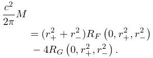
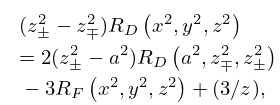
5: 19.22 Quadratic Transformations

… ►

19.22.4 $$(p_{\pm }^2-p_{\mp }^2)R_J(0,x^2,y^2,p^2)=2(p_{\pm }^2-a^2)R_J(0,xy,a^2,p_{\pm }^2)-3R_F(0,xy,a^2)+3\pi /(2p),$$

ⓘ

Symbols:

$R_F(x,y,z)$: symmetric elliptic integral of first kind, $R_J(x,y,z,p)$: symmetric elliptic integral of third kind, $\pi$: the ratio of the circumference of a circle to its diameter and $p_{\pm }$: modified parameter

Referenced by:

§19.22(i), §19.22(i)

Permalink:

http://dlmf.nist.gov/19.22.E4

Encodings:

pMML, png, TeX

See also:

Annotations for §19.22(i), §19.22 and Ch.19

… ►If the last variable of $R_J$ is negative, then the Cauchy principal value is … ►

$2z_{\pm }=\sqrt{(z+x)(z+y)}\pm \sqrt{(z-x)(z-y)},$

… ►

19.22.19 $$(z_{\pm }^2-z_{\mp }^2)R_D(x^2,y^2,z^2)=2(z_{\pm }^2-a^2)R_D(a^2,z_{\mp }^2,z_{\pm }^2)-3R_F(x^2,y^2,z^2)+(3/z),$$

ⓘ

Symbols:

$R_D(x,y,z)$: elliptic integral symmetric in only two variables and $R_F(x,y,z)$: symmetric elliptic integral of first kind

Referenced by:

§19.22(iii), §19.22(iii), §19.36(ii)

Permalink:

http://dlmf.nist.gov/19.22.E19

Encodings:

pMML, png, TeX

See also:

Annotations for §19.22(iii), §19.22 and Ch.19

… ►However, if $x$ and $y$ are complex conjugates and $z$ and $p$ are real, then the right-hand sides of all transformations in §§19.22(i) and 19.22(iii)—except (19.22.3) and (19.22.22)—are free of complex numbers and $p_{\pm }^2-p_{\mp }^2=\pm |p^2-x^2|\ne 0$. …

6: 33.21 Asymptotic Approximations for Large $|r|$

… ►We indicate here how to obtain the limiting forms of $f(ϵ,\mathrm{\ell };r)$, $h(ϵ,\mathrm{\ell };r)$, $s(ϵ,\mathrm{\ell };r)$, and $c(ϵ,\mathrm{\ell };r)$ as $r\to \pm \mathrm{\infty }$, with $ϵ$ and $\mathrm{\ell }$ fixed, in the following cases: ►

When $r\to \pm \mathrm{\infty }$ with $ϵ>0$, Equations (33.16.4)–(33.16.7) are combined with (33.10.1).

►

When $r\to \pm \mathrm{\infty }$ with , Equations (33.16.10)–(33.16.13) are combined with

33.21.1

${\zeta }_{\mathrm{\ell }}(\nu ,r)\sim {\mathrm{e}}^{-r/\nu }{(2r/\nu )}^{\nu },$

${\xi }_{\mathrm{\ell }}(\nu ,r)\sim {\mathrm{e}}^{r/\nu }{(2r/\nu )}^{-\nu }$ , $r\to \mathrm{\infty }$,

ⓘ

Symbols:

$\sim$: asymptotic equality, $\mathrm{e}$: base of natural logarithm, $\mathrm{\ell }$: nonnegative integer, $r$: real variable, $\nu$: parameter, ${\zeta }_{\mathrm{\ell }}(\nu ,r)$: function and ${\xi }_{\mathrm{\ell }}(\nu ,r)$: function

Permalink:

http://dlmf.nist.gov/33.21.E1

Encodings:

pMML, pMML, png, png, TeX, TeX

See also:

Annotations for §33.21(i), §33.21 and Ch.33

33.21.2

${\zeta }_{\mathrm{\ell }}(-\nu ,r)\sim {\mathrm{e}}^{r/\nu }{(-2r/\nu )}^{-\nu },$

${\xi }_{\mathrm{\ell }}(-\nu ,r)\sim {\mathrm{e}}^{-r/\nu }{(-2r/\nu )}^{\nu },$ $r\to -\mathrm{\infty }$.

ⓘ

Symbols:

$\sim$: asymptotic equality, $\mathrm{e}$: base of natural logarithm, $\mathrm{\ell }$: nonnegative integer, $r$: real variable, $\nu$: parameter, ${\zeta }_{\mathrm{\ell }}(\nu ,r)$: function and ${\xi }_{\mathrm{\ell }}(\nu ,r)$: function

Permalink:

http://dlmf.nist.gov/33.21.E2

Encodings:

pMML, pMML, png, png, TeX, TeX

See also:

Annotations for §33.21(i), §33.21 and Ch.33

Corresponding approximations for $s(ϵ,\mathrm{\ell };r)$ and $c(ϵ,\mathrm{\ell };r)$ as $r\to \mathrm{\infty }$ can be obtained via (33.16.17), and as $r\to -\mathrm{\infty }$ via (33.16.18).

►

When $r\to \pm \mathrm{\infty }$ with $ϵ=0$, combine (33.20.1), (33.20.2) with §§10.7(ii), 10.30(ii).

… ►For asymptotic expansions of $f(ϵ,\mathrm{\ell };r)$ and $h(ϵ,\mathrm{\ell };r)$ as $r\to \pm \mathrm{\infty }$ with $ϵ$ and $\mathrm{\ell }$ fixed, see Curtis (1964a, §6).

7: 12.19 Tables

… ►

Abramowitz and Stegun (1964, Chapter 19) includes $U(a,x)$ and $V(a,x)$ for $\pm a=0(.1)1(.5)5$, $x=0(.1)5$, 5S; $W(a,\pm x)$ for $\pm a=0(.1)1(1)5$, $x=0(.1)5$, 4-5D or 4-5S.

… ►

Kireyeva and Karpov (1961) includes $D_p\left(x(1+\mathrm{i})\right)$ for $\pm x=0(.1)5$, $p=0(.1)2$, and $\pm x=5(.01)10$, $p=0(.5)2$, 7D.

►

Karpov and Čistova (1964) includes $D_p\left(x\right)$ for $p=-2(.1)0$, $\pm x=0(.01)5$; $p=-2(.05)0$, $\pm x=5(.01)10$, 6D.

… ►

Zhang and Jin (1996, pp. 455–473) includes $U(\pm n-\frac{1}{2},x)$, $V(\pm n-\frac{1}{2},x)$, $U(\pm \nu -\frac{1}{2},x)$, $V(\pm \nu -\frac{1}{2},x)$, and derivatives, $\nu =n+\frac{1}{2}$, $n=0(1)10(10)30$, $x=0.5,1,5,10,30,50$, 8S; $W(a,\pm x)$, $W(-a,\pm x)$, and derivatives, $a=h(1)5+h$, $x=0.5,1$ and $a=h(1)5+h$, $x=5$, $h=0,0.5$, 8S. Also, first zeros of $U(a,x)$, $V(a,x)$, and of derivatives, $a=-6(.5)-1$, 6D; first three zeros of $W(a,-x)$ and of derivative, $a=0(.5)4$, 6D; first three zeros of $W(-a,\pm x)$ and of derivative, $a=0.5(.5)5.5$, 6D; real and imaginary parts of $U(a,z)$, $a=-1.5(1)1.5$, $z=x+\mathrm{i}y$, $x=0.5,1,5,10$, $y=0(.5)10$, 8S.

…

8: 26.18 Counting Techniques

… ►Then the number of elements in the set $S\setminus (A_1\cup A_2\cup \mathrm{\cdots }\cup A_n)$ is ►

26.18.1

ⓘ

Symbols:

$\left|A\right|$: number of elements of a finite set $A$ , $\cap$: intersection, $\setminus$: set subtraction, $\cup$: union, $j$: nonnegative integer, $n$: nonnegative integer, $A_k$: subsets and $S$: set

Permalink:

http://dlmf.nist.gov/26.18.E1

Encodings:

pMML, png, TeX

See also:

Annotations for §26.18 and Ch.26

… ►

26.18.3 $$n!+\sum _{t=1}^n{(-1)}^t{r}_t(B)(n-t)!.$$

ⓘ

Symbols:

$!$: factorial (as in $n!$), $n$: nonnegative integer, $r_j(B)$: number of rook positions and $B$: subset

Permalink:

http://dlmf.nist.gov/26.18.E3

Encodings:

pMML, png, TeX

See also:

Annotations for §26.18, §26.18 and Ch.26

…

9: 11.8 Analogs to Kelvin Functions

§11.8 Analogs to Kelvin Functions

►For properties of Struve functions of argument $x{\mathrm{e}}^{\pm 3\pi \mathrm{i}/4}$ see McLachlan and Meyers (1936).

10: 4.16 Elementary Properties

… ►

Table 4.16.2: Trigonometric functions: quarter periods and change of sign.

► ►►►►►►

$x$	$-\theta$	$\frac{1}{2}\pi \pm \theta$	$\pi \pm \theta$	$\frac{3}{2}\pi \pm \theta$	$2\pi \pm \theta$
$\sin x$	$-\sin \theta$	$\cos \theta$	$\mp \sin \theta$	$-\cos \theta$	$\pm \sin \theta$
$\cos x$	$\cos \theta$	$\mp \sin \theta$	$-\cos \theta$	$\pm \sin \theta$	$\cos \theta$
$\tan x$	$-\tan \theta$	$\mp \cot \theta$	$\pm \tan \theta$	$\mp \cot \theta$	$\pm \tan \theta$
…
$\cot x$	$-\cot \theta$	$\mp \tan \theta$	$\pm \cot \theta$	$\mp \tan \theta$	$\pm \cot \theta$

►

…