.2014年世界杯朝鲜战绩『网址:mxsty.cc』.世界杯1998假球-m6q3s2-2022年11月30日9时27分4秒

SearchAdvancedHelp

Did you mean .2014年世界杯朝鲜战绩『网址:style』.世界杯1998假球-m6q3s2-2022年11月30日9时27分4秒 ?

(0.006 seconds)

1—10 of 539 matching pages

1: 13.30 Tables

… ►

Žurina and Osipova (1964) tabulates $M(a,b,x)$ and $U(a,b,x)$ for $b=2$, $a=-0.98(.02)1.10$, $x=0(.01)4$, 7D or 7S.

►

Slater (1960) tabulates $M(a,b,x)$ for $a=-1(.1)1$, $b=0.1(.1)1$, and $x=0.1(.1)10$, 7–9S; $M(a,b,1)$ for $a=-11(.2)2$ and $b=-4(.2)1$, 7D; the smallest positive $x$-zero of $M(a,b,x)$ for $a=-4(.1)-0.1$ and $b=0.1(.1)2.5$, 7D.

… ►

Zhang and Jin (1996, pp. 411–423) tabulates $M(a,b,x)$ and $U(a,b,x)$ for $a=-5(.5)5$, $b=0.5(.5)5$, and $x=0.1,1,5,10,20,30$, 8S (for $M(a,b,x)$) and 7S (for $U(a,b,x)$).

…

2: 24.2 Definitions and Generating Functions

… ►

Table 24.2.1: Bernoulli and Euler numbers.

► ►►►

$n$	$B_n$	$E_n$
…
$4$	$-\frac{1}{30}$	$5$
…

►

… ►

Table 24.2.3: Bernoulli numbers $B_n=N/D$.

► ►►►

$n$	$N$	$D$	$B_n$
…
$4$	$-1$	$30$	$-\mathrm{3.33333\hspace{0.33em}3333}$	$\mathrm{\times 10⁻²}$
…

►

… ►

Table 24.2.5: Coefficients $b_{n,k}$ of the Bernoulli polynomials $B_n\left(x\right)={\sum }_{k=0}^n{b}_{n,k}{x}^k$.

► ►►►

	$k$
$n$	$0$	$1$	$2$	$3$	$4$	$5$	$6$	$7$	$8$	$9$	$10$	$11$	$12$	$13$	$14$	$15$
…

►

►

Table 24.2.6: Coefficients $e_{n,k}$ of the Euler polynomials $E_n\left(x\right)={\sum }_{k=0}^n{e}_{n,k}{x}^k$.

► ►►►►

	$k$
$n$	$0$	$1$	$2$	$3$	$4$	$5$	$6$	$7$	$8$	$9$	$10$	$11$	$12$	$13$	$14$	$15$
…
$11$	$\frac{691}{4}$	$0$	$-\frac{1705}{2}$	$0$	$\frac{2805}{4}$	$0$	$-231$	$0$	$\frac{165}{4}$	$0$	$-\frac{11}{2}$	$1$
…

►

3: 26.2 Basic Definitions

… ►If, for example, a permutation of the integers 1 through 6 is denoted by $256413$, then the cycles are $\left(1,2,5\right)$, $\left(3,6\right)$, and $\left(4\right)$. …The function $\sigma$ also interchanges 3 and 6, and sends 4 to itself. … ►As an example, $\{1,3,4\}$, $\{2,6\}$, $\{5\}$ is a partition of $\{1,2,3,4,5,6\}$. … ►As an example, $\{1,1,1,2,4,4\}$ is a partition of 13. … ►The example $\{1,1,1,2,4,4\}$ has six parts, three of which equal 1. …

4: Staff

… ►

Richard B. Paris, University of Abertay, Chaps. 8, 11

… ►

Ranjan Roy, Beloit College, Beloit, Chaps. 1, 4, 5

… ►

Hans Volkmer, University of Wisconsin, Milwaukee, Chaps. 29, 30

… ►

Richard B. Paris, University of Abertay Dundee, for Chaps. 8, 11 (deceased)

… ►

Hans Volkmer, University of Wisconsin–Milwaukee, for Chaps. 29, 30

…

5: 26.9 Integer Partitions: Restricted Number and Part Size

… ►

Table 26.9.1: Partitions $p_k\left(n\right)$.

► ►►►►►

$n$	$k$
	…
6	0	1	4	7	9	10	11	11	11	11	11
7	0	1	4	8	11	13	14	15	15	15	15
…
9	0	1	5	12	18	23	26	28	29	30	30
…

►

… ►

…

Figure 26.9.1: Ferrers graph of the partition $7+4+3+3+2+1$.

… ►The conjugate to the example in Figure 26.9.1 is $6+5+4+2+1+1+1$. …

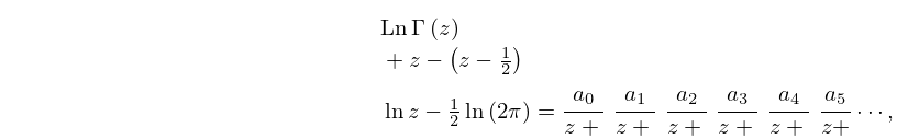
6: 5.10 Continued Fractions

… ►

5.10.1 $$\mathrm{Ln}\mathrm{\Gamma }\left(z\right)+z-\left(z-\frac{1}{2}\right)\ln z-\frac{1}{2}\ln \left(2\pi \right)=\frac{a_0}{z+}\frac{a_1}{z+}\frac{a_2}{z+}\frac{a_3}{z+}\frac{a_4}{z+}\frac{a_5}{z+}\mathrm{\cdots },$$

ⓘ

Symbols:

$\mathrm{\Gamma }\left(z\right)$: gamma function, $\pi$: the ratio of the circumference of a circle to its diameter, $\mathrm{Ln}z$: general logarithm function, $\ln z$: principal branch of logarithm function, $z$: complex variable and $a_k$: coefficient

Referenced by:

Erratum (V1.0.10) for Equations (5.9.10), (5.9.11), (5.10.1), (5.11.1), (5.11.8)

Permalink:

http://dlmf.nist.gov/5.10.E1

Encodings:

pMML, png, TeX

Addition (effective with 1.0.10):

To increase the region of validity of this equation, the logarithm of the gamma function that appears on its left-hand side has been changed to $\mathrm{Ln}\mathrm{\Gamma }\left(z\right)$, where $\mathrm{Ln}$ is the general logarithm. Originally $\ln \mathrm{\Gamma }\left(z\right)$ was used, where $\ln$ is the principal branch of the logarithm.

Suggested 2015-02-13 by Philippe Spindel

See also:

Annotations for §5.10 and Ch.5

… ►

$a_1=\frac{1}{30},$

… ►

$a_4=\frac{22999}{22737},$

… ►For exact values of $a_7$ to $a_{11}$ and 40S values of $a_0$ to $a_{40}$, see Char (1980). …

7: 8.26 Tables

… ►

Zhang and Jin (1996, Table 3.8) tabulates $\gamma (a,x)$ for $a=0.5,1,3,5,10,25,50,100$, $x=0(.1)1(1)3,5(5)30,50,100$ to 8D or 8S.

… ►

Pearson (1968) tabulates $I_x(a,b)$ for $x=0.01(.01)1$, $a,b=0.5(.5)11(1)50$, with $b\le a$, to 7D.

… ►

Abramowitz and Stegun (1964, pp. 245–248) tabulates $E_n\left(x\right)$ for $n=2,3,4,10,20$, $x=0(.01)2$ to 7D; also $(x+n){\mathrm{e}}^x{E}_n\left(x\right)$ for $n=2,3,4,10,20$, $x^{-1}=0(.01)0.1(.05)0.5$ to 6S.

… ►

Zhang and Jin (1996, Table 19.1) tabulates $E_n\left(x\right)$ for $n=1,2,3,5,10,15,20$, $x=0(.1)1,1.5,2,3,5,10,20,30,50,100$ to 7D or 8S.

8: 6.19 Tables

… ►

Abramowitz and Stegun (1964, Chapter 5) includes $x^{-1}\mathrm{Si}\left(x\right)$, $-x^{-2}\mathrm{Cin}\left(x\right)$, $x^{-1}\mathrm{Ein}\left(x\right)$, $-x^{-1}\mathrm{Ein}\left(-x\right)$, $x=0(.01)0.5$; $\mathrm{Si}\left(x\right)$, $\mathrm{Ci}\left(x\right)$, $\mathrm{Ei}\left(x\right)$, $E_1\left(x\right)$, $x=0.5(.01)2$; $\mathrm{Si}\left(x\right)$, $\mathrm{Ci}\left(x\right)$, $x{\mathrm{e}}^{-x}\mathrm{Ei}\left(x\right)$, $x{\mathrm{e}}^x{E}_1\left(x\right)$, $x=2(.1)10$; $x\mathrm{f}\left(x\right)$, $x^2\mathrm{g}\left(x\right)$, $x{\mathrm{e}}^{-x}\mathrm{Ei}\left(x\right)$, $x{\mathrm{e}}^x{E}_1\left(x\right)$, $x^{-1}=0(.005)0.1$; $\mathrm{Si}\left(\pi x\right)$, $\mathrm{Cin}\left(\pi x\right)$, $x=0(.1)10$. Accuracy varies but is within the range 8S–11S.

►

Zhang and Jin (1996, pp. 652, 689) includes $\mathrm{Si}\left(x\right)$, $\mathrm{Ci}\left(x\right)$, $x=0(.5)20(2)30$, 8D; $\mathrm{Ei}\left(x\right)$, $E_1\left(x\right)$, $x=[0,100]$, 8S.

… ►

Abramowitz and Stegun (1964, Chapter 5) includes the real and imaginary parts of $z{\mathrm{e}}^z{E}_1\left(z\right)$, $x=-19(1)20$, $y=0(1)20$, 6D; ${\mathrm{e}}^z{E}_1\left(z\right)$, $x=-4(.5)-2$, $y=0(.2)1$, 6D; $E_1\left(z\right)+\ln z$, $x=-2(.5)2.5$, $y=0(.2)1$, 6D.

►

Zhang and Jin (1996, pp. 690–692) includes the real and imaginary parts of $E_1\left(z\right)$, $\pm x=0.5,1,3,5,10,15,20,50,100$, $y=0(.5)1(1)5(5)30,50,100$, 8S.

9: Publications

… ►

Interactive 3D Visualization of Mathematical Functions Using VRML, Technical Report NISTIR 6289 (February 1999), National Institute of Standards and Technology.

… ►

Boundary/Contour Fitted Grid Generation for Effective Visualizations in a Digital Library of Mathematical Functions, Proceedings of the 9th International Conference on Numerical Grid Generation in Computational Field Simulations, San Jose, June 11–18, 2005. pp. 61–71.

►

Web-Based 3D Visualization in a Digital Library of Mathematical Functions, Proceedings of the Web3D Symposium, Bangor, UK, March 29–April 1, 2005.

… ►

Methods of Relevance Ranking and Hit-content Generation in Math Search, Proceedings of Mathematical Knowledge Management (MKM2007), RISC, Hagenberg, Austria, June 27–30, 2007.

…

10: 11 Struve and Related Functions

Chapter 11 Struve and Related Functions

…