.11选5世界杯电竞网址『世界杯佣金分红55%，咨询专员：@ky975』.4y0.k2q1w9-2022年11月29日8时51分48秒6qguwmgqc

Did you mean .11选5世界杯电竞网址『世界杯佣金分红55%，咨询专员：@1975』.4y0.k2q1w9-2022年11月29日8时51分48秒6qguwmgqc ?

(0.006 seconds)

1—10 of 349 matching pages

1: 13.30 Tables

… ►

•

Slater (1960) tabulates $M\left(a,b,x\right)$ for $a=-1(.1)1$ , $b=0.1(.1)1$ , and $x=0.1(.1)10$ , 7–9S; $M\left(a,b,1\right)$ for $a=-11(.2)2$ and $b=-4(.2)1$ , 7D; the smallest positive $x$ -zero of $M\left(a,b,x\right)$ for $a=-4(.1){-}0.1$ and $b=0.1(.1)2.5$ , 7D.

… ►

•

Zhang and Jin (1996, pp. 411–423) tabulates $M\left(a,b,x\right)$ and $U\left(a,b,x\right)$ for $a=-5(.5)5$ , $b=0.5(.5)5$ , and $x=0.1,1,5,10,20,30$ , 8S (for $M\left(a,b,x\right)$ ) and 7S (for $U\left(a,b,x\right)$ ).

…

2: 25.20 Approximations

… ►

•

Cody et al. (1971) gives rational approximations for $\zeta\left(s\right)$ in the form of quotients of polynomials or quotients of Chebyshev series. The ranges covered are $0.5\leq s\leq 5$ , $5\leq s\leq 11$ , $11\leq s\leq 25$ , $25\leq s\leq 55$ . Precision is varied, with a maximum of 20S.

►

•

Piessens and Branders (1972) gives the coefficients of the Chebyshev-series expansions of $s\zeta\left(s+1\right)$ and $\zeta\left(s+k\right)$ , $k=2,3,4,5,8$ , for $0\leq s\leq 1$ (23D).

… ►

•

Antia (1993) gives minimax rational approximations for $\Gamma\left(s+1\right)F_{s}(x)$ , where $F_{s}(x)$ is the Fermi–Dirac integral (25.12.14), for the intervals $-\infty<x\leq 2$ and $2\leq x<\infty$ , with $s=-\frac{1}{2},\frac{1}{2},\frac{3}{2},\frac{5}{2}$ . For each $s$ there are three sets of approximations, with relative maximum errors $10^{-4},10^{-8},10^{-12}$ .

3: 26.2 Basic Definitions

… ►If, for example, a permutation of the integers 1 through 6 is denoted by

256413

, then the cycles are

{\left(1,2,5\right)}

{\left(3,6\right)}

, and

{\left(4\right)}

. Here

\sigma(1)=2,\sigma(2)=5

, and

\sigma(5)=1

. … ►As an example,

\{1,3,4\}

\{2,6\}

\{5\}

is a partition of

\{1,2,3,4,5,6\}

. … ►For the actual partitions (

\pi

) for

n=1(1)5

see Table 26.4.1. … ►

Table 26.2.1: Partitions

p\left(n\right)

► ►►►

$n$	$p\left(n\right)$	$n$	$p\left(n\right)$	$n$	$p\left(n\right)$
…
4	5	21	792	38	26015
…

►

4: 8.26 Tables

… ►

•

Pearson (1965) tabulates the function $I(u,p)$ ( $=P\left(p+1,u\right)$ ) for $p=-1(.05)0(.1)5(.2)50$ , $u=0(.1)u_{p}$ to 7D, where $I(u,u_{p})$ rounds off to 1 to 7D; also $I(u,p)$ for $p=-0.75(.01)-1$ , $u=0(.1)6$ to 5D.

►

•

Zhang and Jin (1996, Table 3.8) tabulates $\gamma\left(a,x\right)$ for $a=0.5,1,3,5,10,25,50,100$ , $x=0(.1)1(1)3,5(5)30,50,100$ to 8D or 8S.

… ►

•

Zhang and Jin (1996, Table 3.9) tabulates $I_{x}\left(a,b\right)$ for $x=0(.05)1$ , $a=0.5,1,3,5,10$ , $b=1,10$ to 8D.

… ►

•

Stankiewicz (1968) tabulates $E_{n}\left(x\right)$ for $n=1(1)10$ , $x=0.01(.01)5$ to 7D.

►

•

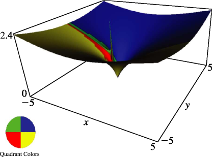
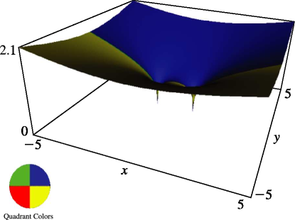
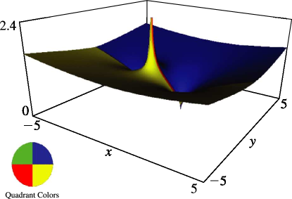
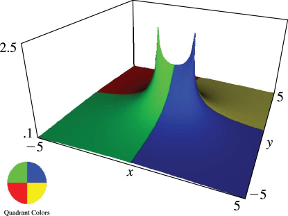
Zhang and Jin (1996, Table 19.1) tabulates $E_{n}\left(x\right)$ for $n=1,2,3,5,10,15,20$ , $x=0(.1)1,1.5,2,3,5,10,20,30,50,100$ to 7D or 8S.

5: 14.22 Graphics

… ►

See accompanying text — Figure 14.22.1: $P^{0}_{\ifrac{1}{2}}\left(x+iy\right)$ , $-5\leq x\leq 5$ , $-5\leq y\leq 5$ . … Magnify 3D Help

►

6: 26.9 Integer Partitions: Restricted Number and Part Size

… ►

Table 26.9.1: Partitions

p_{k}\left(n\right)

► ►►►►►

$n$	$k$
$n$	…
4	0	1	3	4	5	5	5	5	5	5	5
5	0	1	3	5	6	7	7	7	7	7	7
…
9	0	1	5	12	18	23	26	28	29	30	30
…

► … ►The conjugate to the example in Figure 26.9.1 is

6+5+4+2+1+1+1

. … ►

Figure 26.9.2: The partition

5+5+3+2

represented as a lattice path.

…

7: 26.13 Permutations: Cycle Notation

… ►

26.13.2

\begin{bmatrix}1&2&3&4&5&6&7&8\\ 3&5&2&4&7&8&1&6\end{bmatrix}

ⓘ

Referenced by:: §26.13, §26.13, §26.13
Permalink:: http://dlmf.nist.gov/26.13.E2
Encodings:: pMML, png, TeX
See also:: Annotations for §26.13 and Ch.26

►is

{\left(1,3,2,5,7\right)}{\left(4\right)}{\left(6,8\right)}

in cycle notation. …In consequence, (26.13.2) can also be written as

{\left(1,3,2,5,7\right)}{\left(6,8\right)}

. … ►For the example (26.13.2), this decomposition is given by

{\left(1,3,2,5,7\right)}{\left(6,8\right)}={\left(1,3\right)}{\left(2,3\right)% }{\left(2,5\right)}{\left(5,7\right)}{\left(6,8\right)}.

… ►Again, for the example (26.13.2) a minimal decomposition into adjacent transpositions is given by

{\left(1,3,2,5,7\right)}{\left(6,8\right)}={\left(2,3\right)}\*{\left(1,2% \right)}\*{\left(4,5\right)}{\left(3,4\right)}{\left(2,3\right)}{\left(3,4% \right)}{\left(4,5\right)}{\left(6,7\right)}{\left(5,6\right)}{\left(7,8\right% )}\*{\left(6,7\right)}

\mathop{\mathrm{inv}}({\left(1,3,2,5,7\right)}{\left(6,8\right)})=11

8: 24.2 Definitions and Generating Functions

… ►

Table 24.2.3: Bernoulli numbers

B_{n}=N/D

► ►►►

$n$	$N$	$D$	$B_{n}$
…
$10$	$5$	$66$	$7.57575\;7576$	$\times 10^{-2}$
…

► ►

Table 24.2.4: Euler numbers

E_{n}

► ►►►

$n$	$E_{n}$
…
$4$	$5$
…

► ►

Table 24.2.5: Coefficients

b_{n,k}

of the Bernoulli polynomials

B_{n}\left(x\right)=\sum_{k=0}^{n}b_{n,k}x^{k}

► ►►►►

	$k$
$n$	$0$	$1$	$2$	$3$	$4$	$5$	$6$	$7$	$8$	$9$	$10$	$11$	$12$	$13$	$14$	$15$
…
$11$	$0$	$\tfrac{5}{6}$	$0$	$-\tfrac{11}{2}$	$0$	$11$	$0$	$-11$	$0$	$\tfrac{55}{6}$	$-\tfrac{11}{2}$	$1$
…

► ►

Table 24.2.6: Coefficients

e_{n,k}

of the Euler polynomials

E_{n}\left(x\right)=\sum_{k=0}^{n}e_{n,k}x^{k}

► ►►►

	$k$
$n$	$0$	$1$	$2$	$3$	$4$	$5$	$6$	$7$	$8$	$9$	$10$	$11$	$12$	$13$	$14$	$15$
…

►

9: 5 Gamma Function

Chapter 5 Gamma Function

…

10: 28.6 Expansions for Small $q$

… ►

28.6.2

a_{1}\left(q\right)=1+q-\tfrac{1}{8}q^{2}-\tfrac{1}{64}q^{3}-\tfrac{1}{1536}q^% {4}+\tfrac{11}{36864}q^{5}+\tfrac{49}{5\;89824}q^{6}+\tfrac{55}{94\;37184}q^{7% }-\tfrac{83}{353\;89440}q^{8}+\cdots,

ⓘ

Symbols:: $a_{\NVar{n}}\left(\NVar{q}\right)$ : eigenvalues of Mathieu equation and $q=h^{2}$ : parameter
Permalink:: http://dlmf.nist.gov/28.6.E2
Encodings:: pMML, png, TeX
See also:: Annotations for §28.6(i), §28.6 and Ch.28

… ►

28.6.10

a_{5}\left(q\right)=25+\tfrac{1}{48}q^{2}+\tfrac{11}{7\;74144}q^{4}+\tfrac{1}{% 1\;47456}q^{5}+\tfrac{37}{8918\;13888}q^{6}+\cdots,

ⓘ

Symbols:: $a_{\NVar{n}}\left(\NVar{q}\right)$ : eigenvalues of Mathieu equation and $q=h^{2}$ : parameter
Permalink:: http://dlmf.nist.gov/28.6.E10
Encodings:: pMML, png, TeX
See also:: Annotations for §28.6(i), §28.6 and Ch.28

►

28.6.11

b_{5}\left(q\right)=25+\tfrac{1}{48}q^{2}+\tfrac{11}{7\;74144}q^{4}-\tfrac{1}{% 1\;47456}q^{5}+\tfrac{37}{8918\;13888}q^{6}+\cdots,

ⓘ

Symbols:: $b_{\NVar{n}}\left(\NVar{q}\right)$ : eigenvalues of Mathieu equation and $q=h^{2}$ : parameter
Permalink:: http://dlmf.nist.gov/28.6.E11
Encodings:: pMML, png, TeX
See also:: Annotations for §28.6(i), §28.6 and Ch.28

… ►For

m=3,4,5,\dots

, … ►For the corresponding expansions of

\operatorname{se}_{m}\left(z,q\right)

for

m=3,4,5,\dots

change

\cos

\sin

everywhere in (28.6.26). …

.11选5世界杯电竞网址『世界杯佣金分红55%，咨询专员：@ky975』.4y0.k2q1w9-2022年11月29日8时51分48秒6qguwmgqc

1—10 of 349 matching pages

1: 13.30 Tables

2: 25.20 Approximations

3: 26.2 Basic Definitions

4: 8.26 Tables

5: 14.22 Graphics

6: 26.9 Integer Partitions: Restricted Number and Part Size

7: 26.13 Permutations: Cycle Notation

8: 24.2 Definitions and Generating Functions

9: 5 Gamma Function

Chapter 5 Gamma Function

10: 28.6 Expansions for Small q

10: 28.6 Expansions for Small $q$