§14.20 Conical (or Mehler) Functions
Contents
- §14.20(i) Definitions and Wronskians
- §14.20(ii) Graphics
- §14.20(iii) Behavior as
- §14.20(iv) Integral Representation
- §14.20(v) Trigonometric Expansion
- §14.20(vi) Generalized Mehler–Fock Transformation
- §14.20(vii) Asymptotic Approximations: Large , Fixed
- §14.20(viii) Asymptotic Approximations: Large ,
- §14.20(ix) Asymptotic Approximations: Large ,
- §14.20(x) Zeros and Integrals
§14.20(i) Definitions and Wronskians
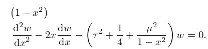
Throughout §14.20 we assume that , with and . (14.2.2) takes the form
| 14.20.1 | |||
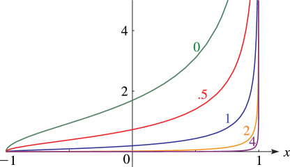
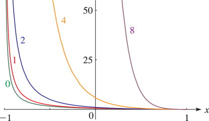
Solutions are known as conical or Mehler functions. For and , a numerically satisfactory pair of real conical functions is and .
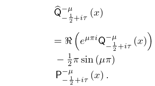
Another real-valued solution of (14.20.1) was introduced in Dunster (1991). This is defined by
| 14.20.2 | |||
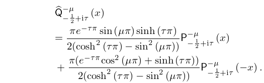
Equivalently,
| 14.20.3 | |||
exists except when and ; compare §14.3(i). It is an important companion solution to when is large; compare §§14.20(vii), 14.20(viii), and 10.25(iii).
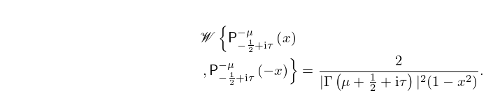
| 14.20.4 | |||
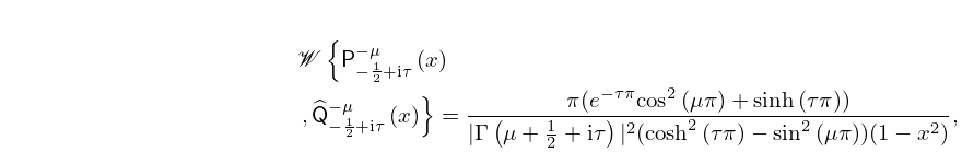
| 14.20.5 | |||
provided that exists.
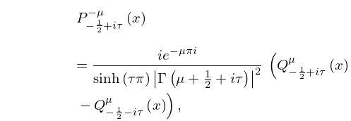
Lastly, for the range , is a real-valued solution of (14.20.1); in terms of (which are complex-valued in general):
| 14.20.6 | |||
| . | |||
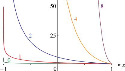
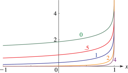
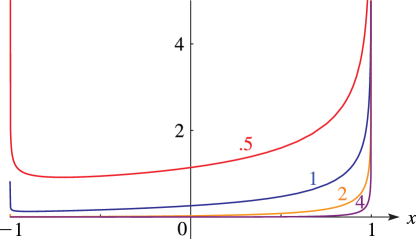
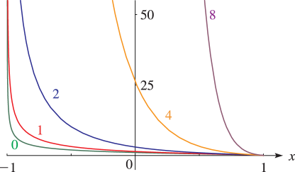
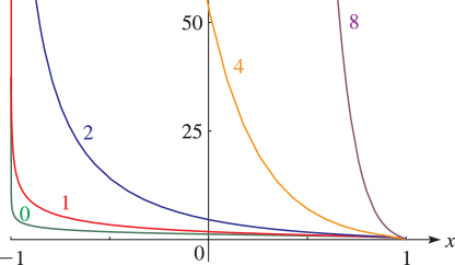
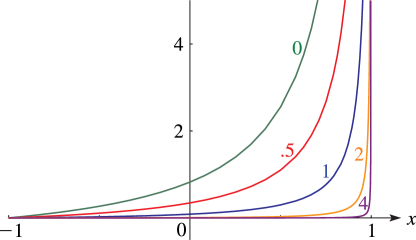
§14.20(ii) Graphics


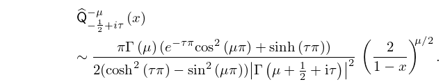
§14.20(iii) Behavior as
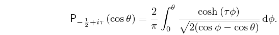
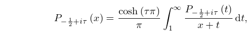
§14.20(iv) Integral Representation
When ,
| 14.20.9 | |||
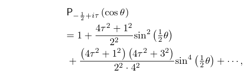
§14.20(v) Trigonometric Expansion
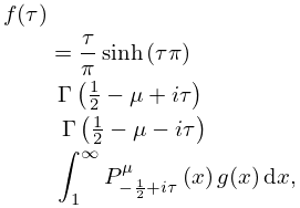
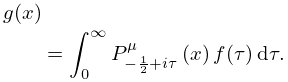
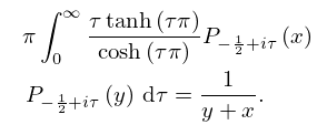
§14.20(vi) Generalized Mehler–Fock Transformation
| 14.20.11 | |||
where
| 14.20.12 | |||
Special cases:
| 14.20.13 | |||
| 14.20.14 | |||
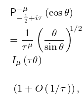
§14.20(vii) Asymptotic Approximations: Large , Fixed
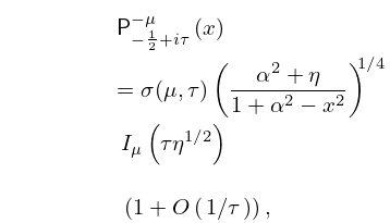
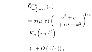
§14.20(viii) Asymptotic Approximations: Large ,
In this subsection and §14.20(ix), and denote arbitrary constants such that and .
As ,
| 14.20.17 | |||
| 14.20.18 | |||
uniformly for and . Here
| 14.20.19 | |||
| 14.20.20 | |||
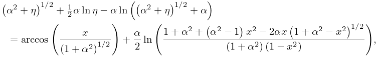
The variable is defined implicitly by
| 14.20.21 | |||
where the inverse trigonometric functions take their principal values. The interval is mapped one-to-one to the interval , with the points and corresponding to and , respectively.
§14.20(ix) Asymptotic Approximations: Large ,
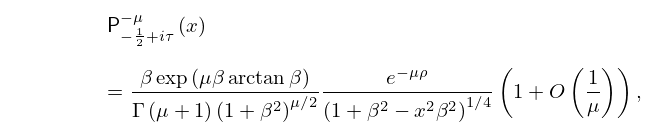
As ,
| 14.20.22 | |||
uniformly for and . Here
| 14.20.23 | |||
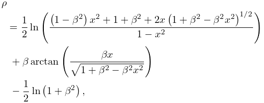
and the variable is defined by
| 14.20.24 | |||
with the inverse tangent taking its principal value. The interval is mapped one-to-one to the interval , with the points , , and corresponding to , , and , respectively.
§14.20(x) Zeros and Integrals
For zeros of see Hobson (1931, §237).
For integrals with respect to involving , see Prudnikov et al. (1990, pp. 218–228).
